


Next: 5.5 Brouncker's Formula For
Up: 5. Area
Previous: 5.3 Monotonic Functions
Index
5.57
Notation ( ,
, ![$A_a^b[f(t){]}$](img1262.gif) .)
.)
Let

be a bounded function from the interval
![$[a,b]$](img1071.gif)
to

. We will denote the area of

by

. Thus
We will sometimes write
![$A_a^b[f(t)]$](img1264.gif)
instead of

. Thus, for example
We will also write
![$I_a^b([f(t)],P)$](img1266.gif)
and
![$O_a^b([f(t)],P)$](img1267.gif)
for

and

respectively.
5.58
Lemma.
5.2
Let

and

be real numbers
such that

and

. Then
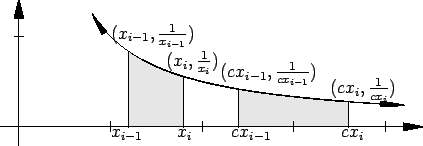
Proof:
Let
 be a partition of
 ![$[a,b]$](img1071.gif) , and let
, and let
be the partition of ![$[ca,cb]$](img1275.gif) obtained by
multiplying the points of
obtained by
multiplying the points of  by
by  .
Then
and
We know that
Hence by (5.59) and (5.60) we have
for every partition  of
of ![$[a,b]$](img1071.gif) . It follows from this and the last statement
of theorem 5.40 that
. It follows from this and the last statement
of theorem 5.40 that
5.61
Exercise.
A
From lemma
5.58 we see that
whenever

, and

. Use this result to show that for

and

![\begin{displaymath}
A_1^{ab}\Big[{1\over t}\Big]=A_1^a\Big[{1\over t}\Big]+A_1^b\Big[{1\over t}\Big].
\end{displaymath}](img1289.gif) |
(5.62) |
5.63
Definition ( .)
.)
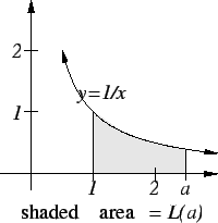
We will define a function

by
By exercise 5.61A we
have
 |
(5.64) |
In this section we will extend the domain of  to all of
 in such a way
that (5.64) holds for all
 .
.
5.65
Theorem.
Let

be real numbers such that

, and let

be a bounded function from
![$[a,b]$](img1071.gif)
to

. Then
 |
(5.66) |
Proof: We want to show
Since
 and the sets
  and
and  are almost
disjoint, this conclusion follows from our assumption about additivity
of area for almost disjoint sets.
I now want to extend the definition of  to cases where
  may be less
than
  . I want equation (5.66) to continue to hold in all cases.
If
  in (5.66), we get
i.e.,
Thus we make the following definition:
5.67
Definition.
Let

be real numbers with

and let

be a bounded
function
from
![$[a,b]$](img1071.gif)
to

. Then we define
5.68
Theorem.
Let

be real numbers and let

be a bounded non-negative real valued function whose
domain contains an interval containing

, and

. Then
Proof: We need to consider the six possible orderings for  and
and  . If
. If
 we already know the result. Suppose
  . Then
 and hence
 , i.e.,
 . The remaining four cases are left as an exercise.
5.69
Exercise.
Prove the remaining four cases of theorem
5.68.
5.70
Definition (Logarithm.)
If

is any positive number, we define the
logarithm of 
by
5.71
Theorem (Properties of Logarithms.) For all
 and all
 we have
Proof: Let
 . From lemma 5.58 we know that if
  then
then
![\begin{displaymath}
A_a^c\Big[ {1\over t}\Big] =A_{ba}^{bc}\Big[{1\over t}\Big]
\end{displaymath}](img1325.gif) |
(5.74) |
If  we get
so equation (5.74) holds in all cases. Let  be arbitrary elements
in
 . Then
Also
so
and it follows from this that
Hence
5.75
Lemma.
For all

,

.
Proof: The proof is by induction on  . For
. For  the lemma is clear.
Suppose
now that the lemma holds for some
 , i.e., suppose that
 .
Then
The lemma now follows by induction.
If
 then
then
 and
and
Thus equation (5.72) holds whenever
 . If
. If
 and
and
 , then
so
Thus (5.72) holds for all  .
. 
5.76
Theorem.
Let

and

be numbers such that

. Then
Proof: By lemma 5.58
Logarithms were first introduced by John
Napier (1550-1632) in 1614. Napier made up the word logarithm from
Greek roots meaning ratio number, and he spent about twenty
years making tables of them.
As far as I have been able to find out, the earliest use of  for
logarithms was by Irving Stringham in
1893[15, vol 2, page 107]. The notation
 is probably more
common among mathematicians than
  , but since calculators almost
always calculate our function with a key called ``ln'', and calculate
something else with a key called ``log'', I have adopted the ``ln''
notation. (Napier did not use any abbreviation for logarithm.)
Logarithms were seen as an important
computational device for reducing multiplications to additions. The first
explicit notice of the fact that logarithms are the same as areas of hyperbolic
segments was made in 1649 by Alfons Anton de Sarasa (1618-1667), and this
observation increased interest in the problem of calculating areas of
hyperbolic segments.
5.77
Entertainment (Calculate  .)
.)
Using any computer or calculator, compute

accurate
to 10 decimal places. You should not make use of any special
functions,
e.g., it is not fair to use the ``ln" key on your calculator.
There are better polygonal
approximations to
![$A_1^2\displaystyle { \Big[{1\over t}\Big]}$](img1352.gif)
than the ones we have
discussed.
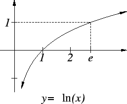
The graph of the logarithm function is shown below.
We know that  and
it is clear that
  is strictly increasing.
If
  , then
From the fact that
 for all
 , it is clear that
 takes on arbitrarily large positive and negative values, but the
function increases
very slowly.
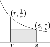
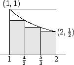
Let
be the regular partition of ![$[1,2]$](img1125.gif) into three subintervals.
Then
into three subintervals.
Then
Now
and
i.e.,
 |
(5.78) |
There is a unique number ![$e\in [2,4]$](img1366.gif) such that
such that  . The uniqueness
is clear because
  is strictly increasing.
The existence of such a number was taken as obvious before the nineteenth
century.
Later we will introduce the intermediate value property
which will allow us to prove that such a number  exists.
For the time being, we will
behave like eighteenth century mathematicians,
and just assert that such a number
  exists.
5.79
Definition ( .)
.)
We
denote the unique number in

whose logarithm is

by

.
5.80
Exercise.
A
Prove that

. (We already know

.)
5.81
Entertainment (Calculate  .)
.)
Using any computing power you have, calculate

as accurately as you
can,
e.g., as a start, find the first digit after the decimal point.


Next: 5.5 Brouncker's Formula For
Up: 5. Area
Previous: 5.3 Monotonic Functions
Index
Ray Mayer
2007-09-07
![]() to cases where
to cases where ![]() may be less
than
may be less
than ![]() . I want equation (5.66) to continue to hold in all cases.
If
. I want equation (5.66) to continue to hold in all cases.
If ![]() in (5.66), we get
in (5.66), we get
![]() and
and ![]() . If
. If
![]() we already know the result. Suppose
we already know the result. Suppose ![]() . Then
. Then
![]() and hence
and hence
![]() , i.e.,
, i.e.,
![]() . The remaining four cases are left as an exercise.
. The remaining four cases are left as an exercise.
![]() . From lemma 5.58 we know that if
. From lemma 5.58 we know that if ![]() then
then
![\begin{eqnarray*}
L(ab)&=&A_1^{ab}\Big[{1\over t}\Big]=A_1^a\Big[{1\over
t}\Big]...
...=&A_1^a\Big[{1\over t}\Big]+A_1^b\Big[{1\over t}\Big]=L(a)+L(b).
\end{eqnarray*}](img1328.gif)
![]() . For
. For ![]() the lemma is clear.
Suppose
now that the lemma holds for some
the lemma is clear.
Suppose
now that the lemma holds for some
![]() , i.e., suppose that
, i.e., suppose that
![]() .
Then
.
Then
![]() then
then
![]() and
and
![]() for
logarithms was by Irving Stringham in
1893[15, vol 2, page 107]. The notation
for
logarithms was by Irving Stringham in
1893[15, vol 2, page 107]. The notation
![]() is probably more
common among mathematicians than
is probably more
common among mathematicians than ![]() , but since calculators almost
always calculate our function with a key called ``ln'', and calculate
something else with a key called ``log'', I have adopted the ``ln''
notation. (Napier did not use any abbreviation for logarithm.)
Logarithms were seen as an important
computational device for reducing multiplications to additions. The first
explicit notice of the fact that logarithms are the same as areas of hyperbolic
segments was made in 1649 by Alfons Anton de Sarasa (1618-1667), and this
observation increased interest in the problem of calculating areas of
hyperbolic segments.
, but since calculators almost
always calculate our function with a key called ``ln'', and calculate
something else with a key called ``log'', I have adopted the ``ln''
notation. (Napier did not use any abbreviation for logarithm.)
Logarithms were seen as an important
computational device for reducing multiplications to additions. The first
explicit notice of the fact that logarithms are the same as areas of hyperbolic
segments was made in 1649 by Alfons Anton de Sarasa (1618-1667), and this
observation increased interest in the problem of calculating areas of
hyperbolic segments.
![$A_1^2\displaystyle { \Big[{1\over t}\Big]}$](img1352.gif) than the ones we have
discussed.
than the ones we have
discussed.
![\begin{eqnarray*}
\ln(2) &=& A_1^2 \Big[{1\over t}\Big] \geq
\alpha(I_1^2(\Big[...
...\over 6} = {1\over 4} + {1\over 5} + {1\over 6} = {37 \over 60}.
\end{eqnarray*}](img1362.gif)
![]() exists.
For the time being, we will
behave like eighteenth century mathematicians,
and just assert that such a number
exists.
For the time being, we will
behave like eighteenth century mathematicians,
and just assert that such a number ![]() exists.
exists.