next up previous index
Next: 6. Limits of Sequences Up: 5. Area Previous: 5.5 Brouncker's Formula For   Index

5.6 Computer Calculation of Area

In this section we will discuss a Maple program for calculating approximate values of $A_a^bf$ for monotonic functions $f$ on the interval $[a,b]$. The programs will be based on formulas discussed in theorem 5.40.

Let $f$ be a decreasing function from the interval $[a,b]$ to $\mbox{{\bf R}}_{\geq 0}$, and let $P=\{x_0,x_1,\cdots ,x_n\}$ be a partition of $[a,b]$. We know that

\begin{displaymath}\alpha(I_a^b(f,P)) \leq A_a^b f \leq \alpha(O_a^b(f,P)),\end{displaymath}

where
$\displaystyle \alpha(I_a^b(f,P))$ $\textstyle =$ $\displaystyle \sum_{i=1}^n (x_i - x_{i-1}) f(x_i),$ (5.83)
$\displaystyle \alpha(O_a^b(f,P))$ $\textstyle =$ $\displaystyle \sum_{i=1}^n (x_i - x_{i-1}) f(x_{i-1}).$ (5.84)

Let $V_a^b(f,P)$ be the average of $\alpha(I_a^b(f,P))$ and $\alpha(O_a^b(f,P))$, so

\begin{displaymath}V_a^b(f,P) = { \alpha(I_a^b(f,P)) + \alpha(O_a^b(f,P)) \over ...
...m_{i=1}^n (x_i - x_{i-1})\cdot{f(x_{i}) + f(x_{i-1}) \over 2}.
\end{displaymath}

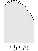
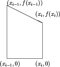
Now $\displaystyle {(x_i - x_{i-1})\cdot{f(x_{i}) + f(x_{x-1}) \over 2}}$ represents the area of the trapezoid with vertices $(x_{i-1},0)$, $(x_{i-1}, f(x_{i-1}))$, $(x_i, f(x_i))$ and $(x_i,0)$, so $V_a^b(f,P)$ represents the area under the polygonal line obtained by joining the points $(x_{i-1}, f(x_{i-1}))$ and $(x_i, f(x_i))$ for $1\leq i\leq n$.

\begin{picture}(2,3)(-.5,-.5)
\put(0,0){\line(1,0){1}}
\put(0,0){\line(0,1){1....
...\put(.8,1.2){$(x_i,f(x_i))$}
\put(0,1.52){$(x_{i-1},f(x_{i-1}))$}
\end{picture}
\psfig{file=ch5i.eps,width=1.5in}

In the programs below, leftsum(f,a,b,n) calculates

\begin{displaymath}\displaystyle {\sum_{j=1}^{n}f\Bigg(a+(j-1)\Big( {{b-a}\over ...
...
\sum_{j=1}^{n}f\Bigg(a+(j-1)\Big( {{b-a}\over n}\Big)\Bigg),\end{displaymath}

which corresponds to (5.84) when $P$ is the regular partition of $[a,b]$ into $n$ equal subintervals, and rightsum(f,a,b,n) calculates

\begin{displaymath}\displaystyle {\sum_{j=1}^n f\Bigg(a+j\Big({{b-a}\over n}\Big...
...n}\Big)
\sum_{j=1}^n f\Bigg(a+j\Big({{b-a}\over n}\Big)\Bigg).\end{displaymath}

which similarly corresponds to (5.83). The command average(f,a,b,n) calculates the average of leftsum(f,a,b,n) and rightsum(f,a,b,n).

The equation of the unit circle is $x^2+y^2=1$, so the upper unit semicircle is the graph of $f$ where $f(x)=\sqrt{1-x^2}$. The area of the unit circle is 4 times the area of the portion of the circle in the first quadrant, so

\begin{displaymath}\pi=4A_0^1[\sqrt{1-t^2}].\end{displaymath}

Also

\begin{displaymath}\ln (2)=A_1^2\Big[{1\over t}\Big].\end{displaymath}

My routines and calculations are given below. Here leftsum, rightsum and average are all procedures with four arguments, f,a,b, and n.

f is a function.

a and b are the endpoints of an interval.

n is the number of subintervals in a partition of [a,b].

The functions F and G are defined by F$(x) = 1/x$ and G $(x) = \sqrt{1-x^2}$. The command

             average(F,1.,2.,10000);
estimates $\ln (2)$ by considering the regular partition of $[1,2]$ into $10000$ equal subintervals. and the command
             4*average(G,0.,1.,2000);
estimates $\pi$ by considering the regular partition of $[0,1]$ into $2000$ equal subintervals.

> leftsum :=
>       (f,a,b,n) -> (b-a)/n*sum(f( a +((j-1)*(b-a))/n),j=1..n);

\begin{displaymath}
{\it leftsum} := ( {f}, {a}, {b}, {n} ) \rightarrow
{\dis...
...)} ( {b} - {a} )}{{n}}}  \! \right)
  \! \right) }{{n}}}
\end{displaymath}

> rightsum := 
>       (f,a,b,n) -> (b-a)/n*sum(f( a +(j*(b-a))/n),j=1..n);

\begin{displaymath}
{\it rightsum} := ( {f}, {a}, {b}, {n} ) \rightarrow
{\di...
...j} ( {b} - {a} )}{{n}}}  \! \right)
  \! \right) }{{n}}}
\end{displaymath}

> average :=
>       (f,a,b,n) -> (leftsum(f,a,b,n) + rightsum(f,a,b,n))/2;

\begin{displaymath}
{\it average} := ( {f}, {a}, {b}, {n} ) \rightarrow
{\dis...
...aystyle \frac {1}{2}} {\rm rightsum}( {f}, {a}, {b
}, {n} )
\end{displaymath}

> F := t -> 1/t;

\begin{displaymath}
{F} := {t} \rightarrow {\displaystyle \frac {1}{{t}}}
\end{displaymath}

> leftsum(F,1.,2.,10000);

\begin{displaymath}
.6931721810
\end{displaymath}

> rightsum(F,1.,2.,10000);

\begin{displaymath}
.6931221810
\end{displaymath}

> average(F,1.,2.,10000);

\begin{displaymath}
.6931471810
\end{displaymath}

> ln(2.);

\begin{displaymath}
.6931471806
\end{displaymath}

> G := t -> sqrt(1-t^2);

\begin{displaymath}
{G} := {t} \rightarrow  {\rm sqrt}( 1 - {t}^{2} )
\end{displaymath}

> 4*leftsum(G,0.,1.,2000);

\begin{displaymath}
3.142579520
\end{displaymath}

> 4*rightsum(G,0.,1.,2000);

\begin{displaymath}
3.140579522
\end{displaymath}

> 4*average(G,0.,1.,2000);

\begin{displaymath}
3.141579521
\end{displaymath}

> evalf(Pi);

\begin{displaymath}
3.141592654
\end{displaymath}

Observe that in these examples, average yields much more accurate approximations than either leftsum or rightsum.


next up previous index
Next: 6. Limits of Sequences Up: 5. Area Previous: 5.5 Brouncker's Formula For   Index
Ray Mayer 2007-09-07