Level Sets and Gradient Flow

Level sets, the gradient, and gradient flow are methods of extracting specific features of a surface. You’ve heard of level sets and the gradient in vector calculus class – level sets show slices of a surface and the gradient shows a sort of 2D “slope” of a surface. These measurements are useful on their own, but they hint at something else, something more abstract. The gradient vectors are perpendicular to the level sets, so will always be in the direction of the “slope” of a point toward a point on a level set. But how would you represent that? The answer is the concept of gradient flow. Read more to learn about how these three standard measurements fit together to flow along a surface, much like a liquid or rolling object.

Level Sets

Consider a function $f : \mathbb{R}^2 \rightarrow \mathbb{R}$. If you were to graph this as a 3D plot, you can visualize how this would turn out to be a cone-like surface, with the small end at 0. This represents the solutions to this equation in three variables. What happens when we want the solutions in two variables, instead? The goal would be to obtain the solutions to this equation at a certain level, meaning at a constant value for one of the variables. Let’s choose $z$. The level set of such a function for a given $z$ is

$$\{ (x,y) \in \mathbb{R}^2 \mid \ f(x,y)=z \}$$

For example, let’s say  $f:(x,y) \mapsto x^2+y^2$. Now we need to pick a few $z$-levels to show the level sets at, say $z\in\{0,1,2,3,4\}$. These level sets turn out to be

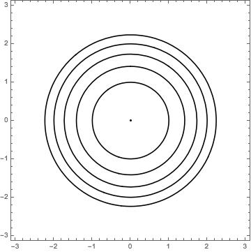
where the circle radius is increasing with $z$-level. All of these level sets turn out to be circles, with one exception being the point at $(0,0)$ – the only solution to $x^2+y^2=0$. Why are the level sets circles when $z>0$? An examination of our function shows that, when you solve for $f$’s level set at $z$, you get an equation of the form $x^2 + y^2 = z$, which is the equation for a circle with radius $\sqrt{z}$. This explains why the circles are getting bigger, but at a decreasing rate; the circle radius is increasing at the rate $\frac{1}{2\sqrt{z}}$. This is an extremely simple example, but it demonstrates level curves, and some following concepts very clearly.

So what are level curves showing? The graph above may have reminded you of something – a contour (or topographical) map of a landscape. Essentially the level sets are the contour lines on a map of a surface. They are cross-sections through the surface, in this case at specific $z$-levels.

The Gradient

The gradient of a scalar function records its partial derivatives throughout its domain. For example, consider a function $f:\mathbb{R}^2 \to \mathbb{R}$. Then,

$$\nabla f : (x,y) \mapsto \left( \frac{\partial f}{\partial x}(x,y), \frac{\partial f}{\partial y}(x,y) \right)$$

is a function $\mathbb{R}^2\to \mathbb{R}^2$.

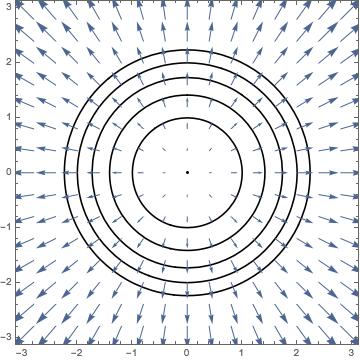
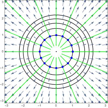
Let’s take a new function $g: (x,y) \mapsto x^2-y^2$ as an example. Since the gradient has range $\mathbb{R}^2$, we can use a vector plot to visualize it, with the level sets for $z\in \{-5,-4,\ldots,4,5\}$ in the background:

What are these gradient arrows representing? It turns out that these arrows show, at each point, which direction yields the largest increase in the value of $g$; the magnitude gives the rate of increase. If you are curious, this is a depiction of $f:(x,y)\mapsto x^2+y^2$’s gradient:

Gradient Flow

These level curves and gradient vector fields are slowly building an outline of a surface in $\mathbb{R}^3$. However, we are still lacking a way of connecting the curves and the arrows. How would one follow the vectors to get from one level curve to the next? With this ability, you could flow across continuously-spaced level curves.

The features we aim to achieve are:

• The flow’s points are solutions to the original function – the flow with be on the surface;
• The flow’s derivative is the gradient – the flow will follow the gradient vectors.

For a point $(x,y)$ in the domain of a function $f:\mathbb{R}^2 \to \mathbb{R}$, the curve that starts at $(x,y)$ and accomplishes this flow is $\gamma_{(x,y)} :\mathbb{R} \rightarrow \mathbb{R}^2$ such that

$$\begin{aligned} \gamma_{(x,y)}(0) &= (x,y) \\ \gamma_{(x,y)}^\prime (t) &= \nabla f (\gamma_{(x,y)} (t)) \end{aligned}$$

As you can see, $\gamma$’s derivative will follow the gradient and $\gamma$ will be centered around a point of “origin” where the flow flows from. What does $\gamma$ look like? Let’s consider gradient flows for our usual functions

$$\begin{aligned} f(x,y) &= x^2 + y^2 \\ g(x,y) &= x^2 - y^2 \end{aligned}$$

$\gamma_{(x,y)}$ of $f$ needs to be a function where

$$\begin{aligned} \gamma_{(x,y)}(t) &\mapsto (x^\prime, y^\prime) \\ \gamma_{(x,y)}(0) &= (x,y) \\ \gamma_{(x,y)}^\prime &= \nabla f (x^\prime, y^\prime) = (2 x^\prime, 2 y^\prime) \end{aligned}$$

Solve this differential equation and you get

$$\gamma_{(x,y)} = (x e^{2t}, y e^{2t})$$

What does $\gamma$ look like? Below are the usual level curves and gradient vector field, and now with the flow lines in green starting at some blue points on the unit circle (we let $t \in [-0.75,0.75]$):

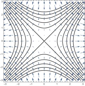
And for $g$, with the same parameters:

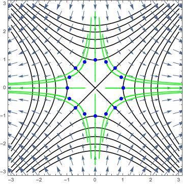
So we have produced gradient flows, and they join the level curves. But what exactly are we visualizing here? One way to think about it is noting that since the gradient is the direction of steepest ascent in the $z$-direction, the reverse of the flow is the path of an object as it rolls on the surface, starting from a high place and rolling down to a lower place (in the exact opposite direction as the gradient vectors point).

To 3D

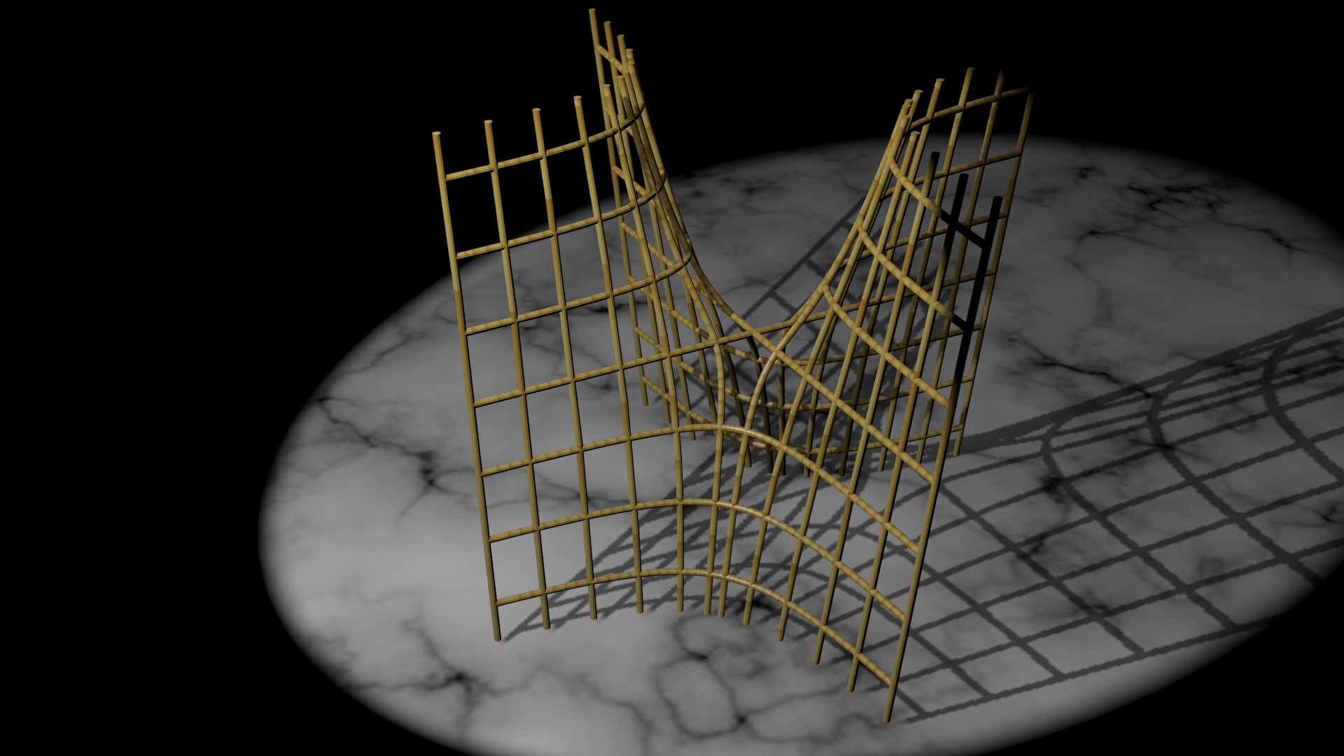
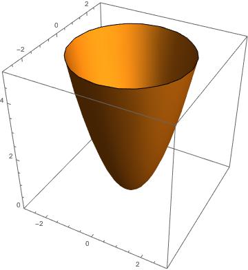
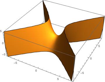
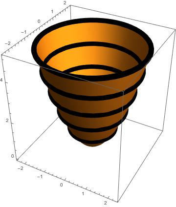
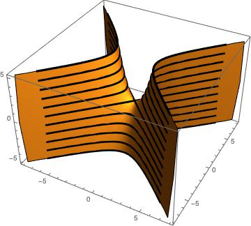
I’ve been showing you 2D pictures of curves and arrows, but the functions that we have been considering are inherently 3D in nature. The functions $f,g$ from above can be visualized as the following parabaloid and saddle surface, respectively:

These shouldn’t be surprising visuals. The level curves, being cross-sections through the surfaces at specified $z$-levels, are only 2D, but they can be fit into this 3D depiction by simply setting the level curves’s $z$-coordinate to its respective $z$-level, highlighted in black:

And finally, the same sort of process can be applied to the flow. We want to preserve the $x,y$ coordinates of the flow, but we need to decide at what $z$-coordinate to put each point on the flow. The natural choice is the following function:

$$\mathrm{flow}_{(x,y)}:t\mapsto ( \gamma_{(x,y)}(t), f( \gamma_{(x,y)} (t)) )$$

There are too many parentheses, but essentially this function plots the flow from before, and assigns its $z$-coordinate to be the value of the original function at the $(x^\prime , y^\prime )$ point that $\gamma$ returns (as a function of $t$, of course). Here are our two favorite functions fully rendered with level (black) and 3D flow lines (orange):

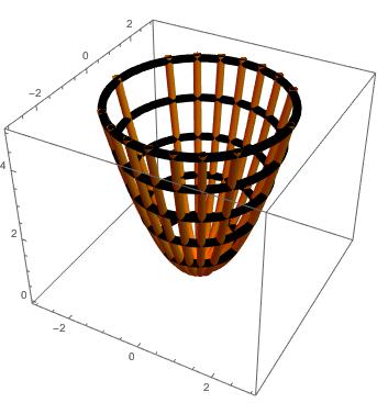
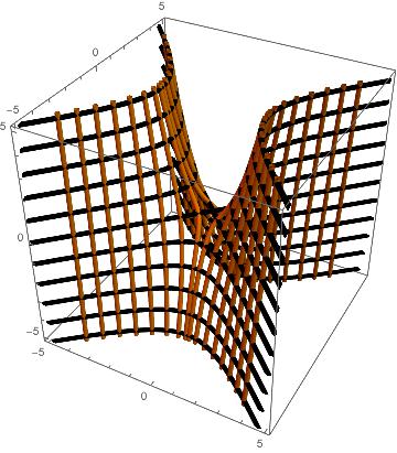
For each, the flow lines originate at points on the $1$-level set, and we let $t$ vary through a large enough interval for the flow lines to fill up the surface. If you imagine looking at these 3D-structures from above, you can confirm that they match the previous 2D graphs. In the parabaloid, you can see that the flow lines converge at the critical point $z=0$, where the level set is a single point. This makes sense intuitively; an object would roll down the slope to the bottom, and come to rest.

As for the saddle, none of the pictured flow lines stop at the critical point (the center of the saddle at $z=0$). There are, in fact, exactly four flow lines that would stop there (they are clearly visible in the 2D depiction in Gradient Flow); the paucity of flow lines going through $g$’s critical point makes that point unstable, a feature I will return to later if this project heads towards Morse theory.

Printing

In the To 3D section, I displayed various 3D models of the concepts I explained. Though these 2D projections on your computer screen are very helpful, physical 3D models can offer a more intuitive and clear expression of the truly 3D surfaces that are concerned. Especially with more complicated models, 3D printing gains a huge advantage of being relatively uncluttered and easily manipulatable.

I am currently working on printing a few different models, and will have updates on their progress in the next two weeks. In the meantime, check out my next article on 3D printing!

← Back to Project Project Home