Iterated Integrals

What is a multiple integral? The notion itself is fairly intuitive: we stretch the notion from single variable calculus of “the area under a function’s graph” to higher dimensions, resulting in the multidimensional analogue of area, volume (or hypervolume). A multiple integral is essentially a way of quantifying the spatial “footprint” that a region or the graph of a function has. It is computable by splitting the region into many smaller pieces, but there is some art to performing this dissection.

Consider a loaf of bread.  One slice of bread has all of the characteristics of bread; that is, we can get a reasonably good picture of the entire loaf from one individual slice. In order, however, to get the full picture we would have to place all the slices next to each other so they re-create the shape of the uncut loaf. It would be much less representative and enlightening, not to mention much more difficult to piece back together, if we cubed the bread. Likewise, we could slice the bread longitudinally, but this would be more difficult to physically cut.

The mathematical analogue to cubing the loaf of bread is the multivariable Riemann Sum. This method partitions each axis and calculates the function’s value on each resulting box. Slicing bread requires more mathematical technology: Fubini’s Theorem. Fubini’s Theorem states, when we have a ‘nice’ function, that the $n$-dimensional multiple integral of this function is the same as the $n$-fold iterated integral; futhermore, this theorem also states that we can use any order of integration, which is to say (in the $2$-dimensional case) that

$$\iint_{[a,b]\times [c,d]}f = \int_{x=a}^{b}\int_{y=c}^{d}f(x,y)=\int_{y=c}^{d}\int_{x=a}^{b}f(x,y)$$

Sometimes it is handy to change order of integration to make an integral easier to compute – this is like cutting bread the standard way, not longitudinally. This commonly occurs when we try to compute the volume of a region $R\subseteq \mathbb{R}^3$ with a triple integral via the formula

$$\mathrm{Vol}(R) = \iiint_R 1$$

For example, consider the region described by $z+\lvert y\rvert\leq \lvert\sin{x}\rvert$. It looks like this: you can manipulate the visualization with your mouse):

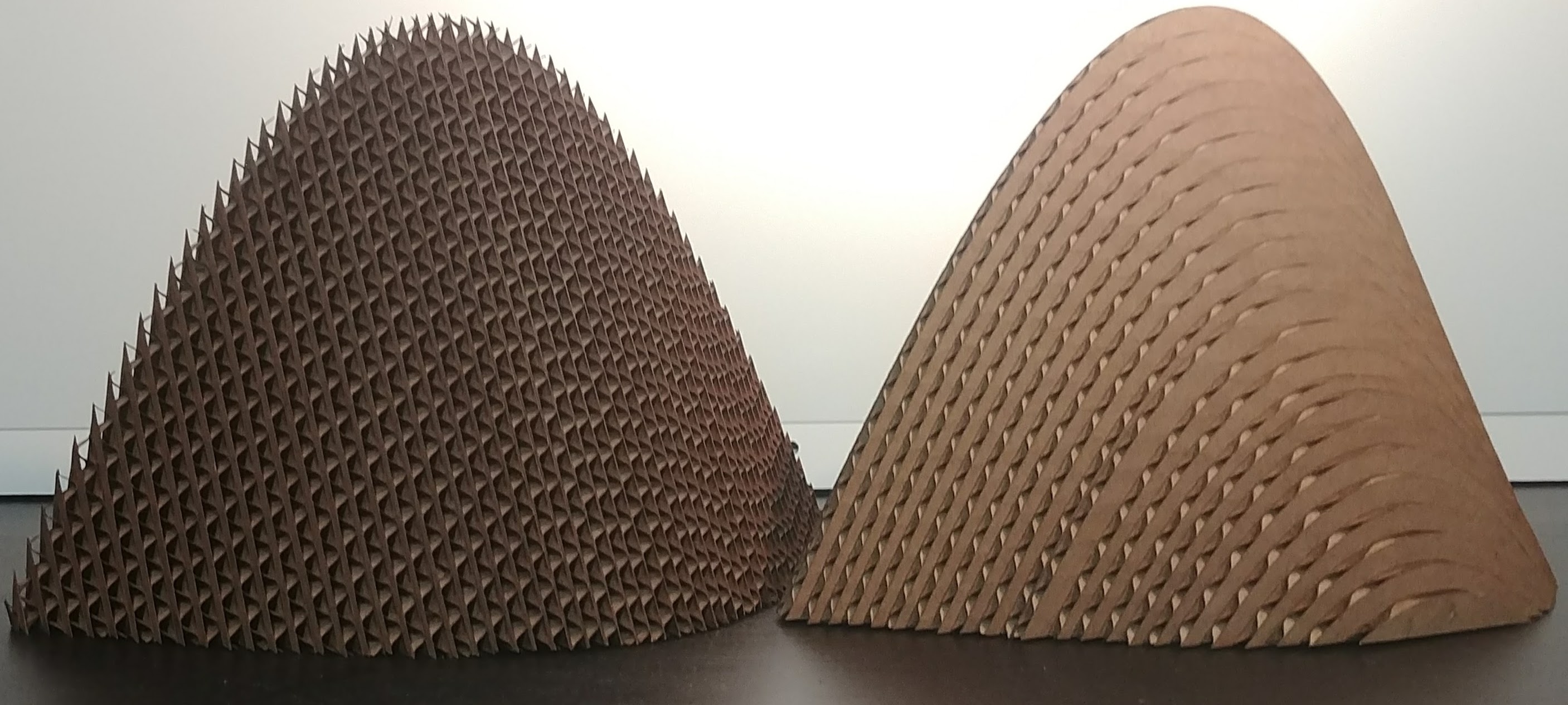
When cut such that the cross sections are in the $xy$- or $xz$-planes we get respectively pointy ellipse-like shapes or parabolic shapes. But, when sliced such that the cross sections are in the $yz$-plane, the entire shape becomes a union of triangles.

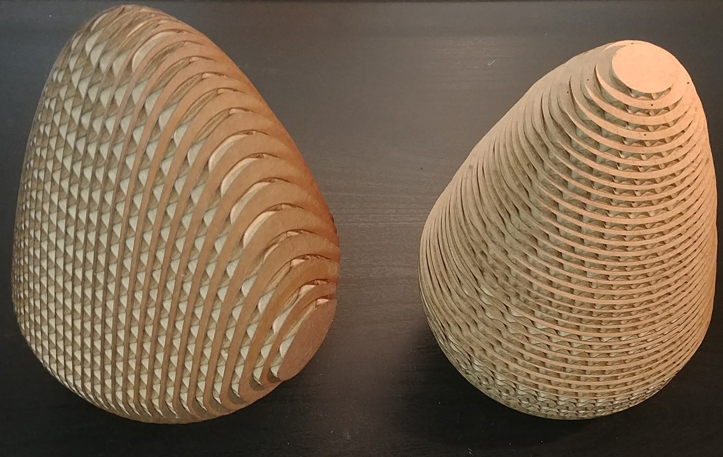
Visual approaches to learning vector calculus help foster an intuitive understanding of the subject matter. While drawing shapes on a blackboard can be helpful for imagining a 3D shape or region, it can also be fiendishly difficult to interpret the 2D projection of a 3D object. Therefore physical sculptures of 3D solids are a useful pedagogical tool, not to mention aesthetically valuable. To construct a sculpture that demonstrates the qualities of iterated integrals I used a laser cutter to cut flat cross sectional slices of a 3D solid which I then constructed. The region described above with a graphic can be seen below displayed in this style of sculpture.  The two sculptures represent different choices of slicing direction, making it clear how some slices are simpler than others.

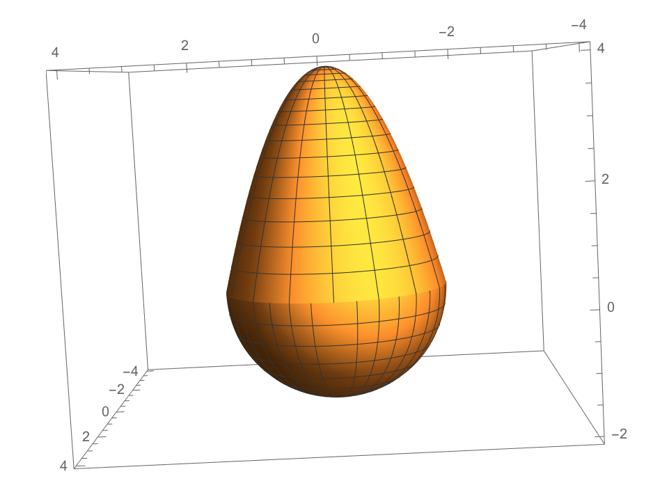
The next example is a shape defined by the following inequality: $x^2+y^2\leq z \leq 4+\sqrt{4-x^2-y^2}$, which is a union of a hemisphere and a parabaloid – a shape that, when viewed from the $xz$- or $yz$-planes, is egg-like, but from the $xy$-plane is a circle.

Cardboard models display the different slicing choices very nicely:

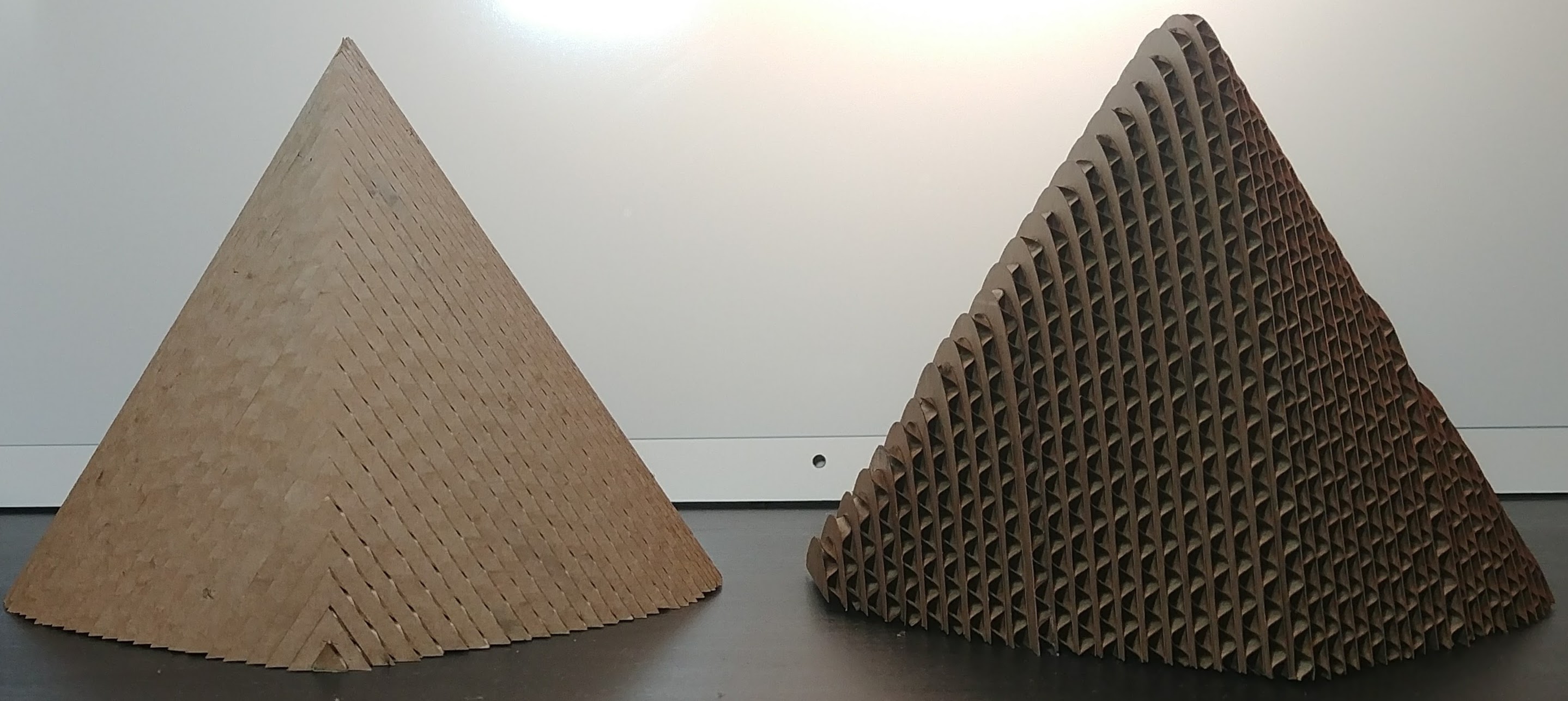
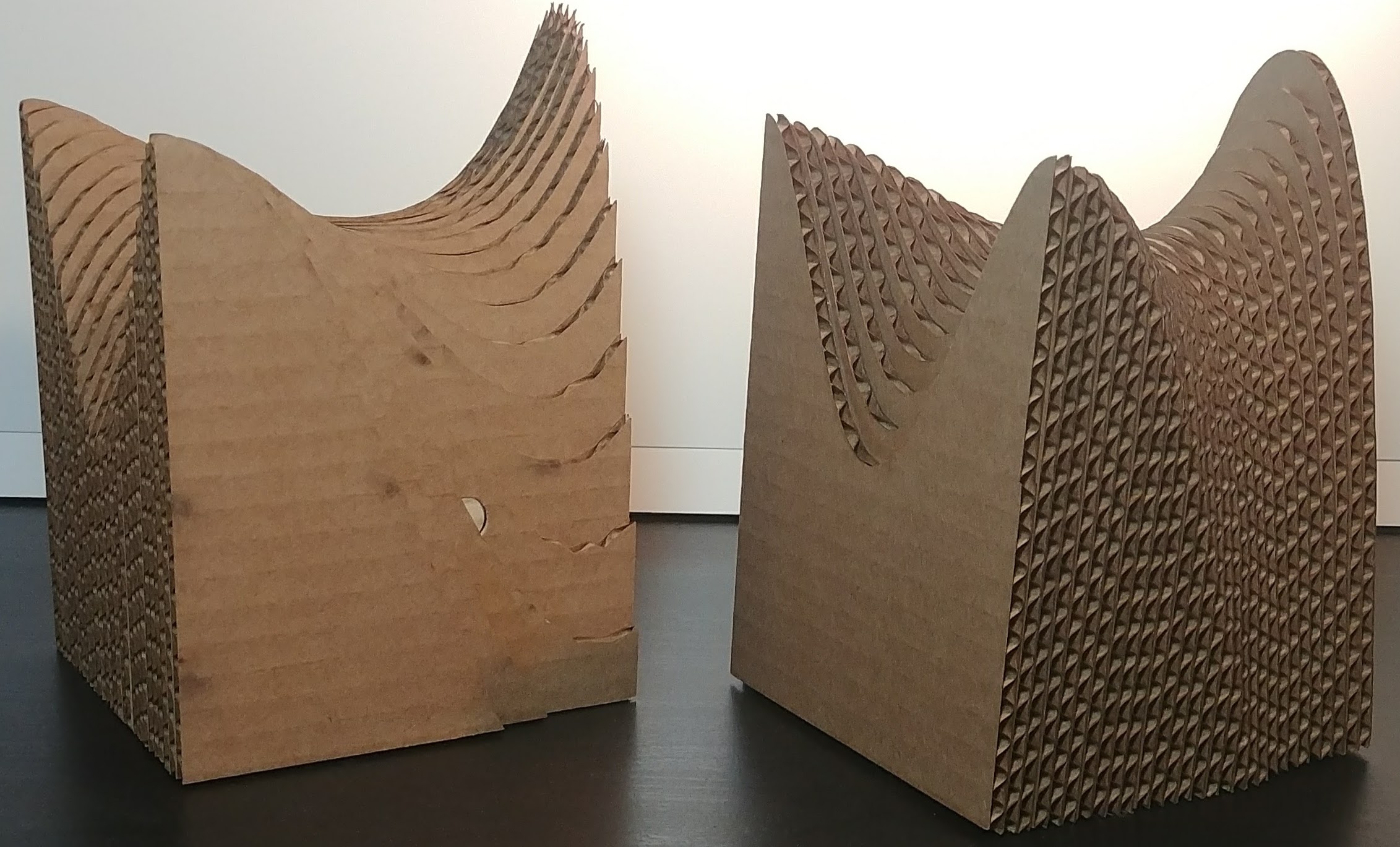
The next shape is the solid that models the region under the graph of the function $f(x,y)=6xy^2-2x^3-3y^4$. This regions looks like this (use your mouse to manipulate the model):

This shape is referred to as a “monkey saddle.” The name is a response to the classical “saddle” shape we get from a graph of $z=x^2-y^2$.

To understand how an iterated integral computing $\iint_{[a,b]\times [c,d]} f$ works, let $g(x)=\int_{y=c}^{d}f(x,y)$. Then we can partition the $[a,b]$ subset of the $x$-axis and take a standard single variable Riemann Sum of the function $g(x)$ to approximate

$\int_{x=a}^b\int_{y=c}^d f(x,y) = \int_{x=a}^b g(x)$ This will look like the left-hand model.  The curves in the $yz$-plane will be smooth, as they have been integrated, but the partitions along the $x$-axis give the model the roughly sliced appearance. Specifically, for this model, the interval $[a,b]$ was partitioned into 29 equal intervals, each of which is the width of a slice of cardboard. The other model, on the right, is an integral of the same function, with the order of integration swapped. That is, let $h(y)=\int_{x=a}^{b}f(x,y)$, then this model displays the Riemann Sum of this function, this time with the curves in the $xz$-plane being smooth.

The method of construction for all of my cardboard sculptures had 3 distinct phases: writing the mathematica code, exporting the mathematica file to software which prepared it for laser cutting, and finally the physical construction. Stay tuned for a blog post which dives into the details of this process!

← Back to Project Project Home