Green’s Theorem

If you are or have been a student of mathematics, physics, or engineering, you have likely encountered the following equation:

$$\oint_C Pdx + Qdy = \iint_D \left ( \frac{\partial Q}{\partial x} - \frac{\partial P }{\partial y} \right )dA$$

This statement, known as Green’s theorem, combines several ideas studied in multi-variable calculus and gives a relationship between curves in the plane and the regions they surround, when embedded in a vector field. While most students are capable of computing these expressions, far fewer have any kind of visual or visceral understanding. In this post, I want to build some of that understanding by discussing each component of the theorem in a visual way. My hope is that, armed with the right intuitions, Green’s theorem should feel nearly natural.

I will assume familiarity with vectors, partial derivatives, and integration.

To begin with, let’s state the theorem properly.

Let $F = (P, Q)$ be a vector field in the plane. Let $C$ be a simple closed curve in the plane which is positively oriented and piecewise smooth, surrounding a region $D$. Then,

$$\oint_C Pdx + Qdy = \iint_D \left ( \frac{\partial Q}{\partial x} - \frac{\partial P }{\partial y} \right )dA$$

In words, the line integral along $C$ of $Pdx + Qdy$ is equal to the double integral over $D$ of $\left ( \frac{\partial Q}{\partial x} - \frac{\partial P }{\partial y} \right )$.

Here’s a picture of what’s going on:

The first thing to notice is the collection of needles on this plane, pointing in various directions. This is a representation of the vector field $F$ permeating this square region of the plane. A vector field is just an assignment of a vector to each point of the plane–a function from points (x, y) to vectors (x, y). Notice that the vectors (needles) are longer towards the right half of the square, showing that the vector field is stronger there. Here is the equation for this vector field:

$$F(x,y) = \left (-\frac{1}{4}y, \frac{3}{4}x \right )$$

The square region here is [0, 1.5] x [0, 1.5].

Embedded in this vector field is a simple, closed curve $C$ (tracing a wedge shape in the plane). It is simple because it doesn’t cross over itself, and closed because it ends where it begins (if one were to walk around it). The curve $C$ encloses a region in the plane we can call $D$. Along this curve runs a ribbon which varies in height, and even dips below the square. This ribbon represents the left expression in Green’s theorem, a line integral. The claim, then, of Green’s theorem is that the total surface area of this ribbon (counting the parts under the square as negative) is equal to this quantity $\left ( \frac{\partial Q}{\partial x} - \frac{\partial P }{\partial y} \right )$ integrated over $D$. We’ll discuss double and line integrals below, but in this example, I have chosen a vector field for which the integrand $\left ( \frac{\partial Q}{\partial x} - \frac{\partial P }{\partial y} \right )$ to be equal to 1, meaning that the ribbon’s area should be equal to the area of the region $D$ enclosed by $C$. An eyeballing of the area of the ribbon and the area of $D$ may convince you that they are indeed equal.

Line Integrals

Let’s look at that vector field again:

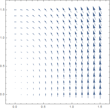
At each point of this region, we have assigned a vector. Imagine that this vector field represents the currents of a river you are crossing (at any given point inside the river, you would feel the current pushing you in some direction). If you crossed this river by following some path, you would feel the currents change and move around you. At times you would feel resisted by the currents and at others you would be helped along. A line integral is a way to add up all these changes in the current as you move along your path, in a way that represents the total resistance you felt along the way. How might we add up this ‘total resistance’? Well, consider that as you move through the vector field, your progress forward (along the path) is only impeded by current in the direction opposite your movement. If the current is at your back, you feel negative resistance. And if the current is perpendicular to your path, it doesn’t affect your forward motion.

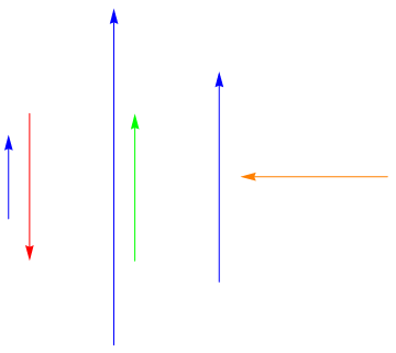
The dot product captures this notion precisely. If two vectors (of unit length) are aligned, their dot product is 1. If they are opposite, it is -1, and if they are perpendicular it is 0. You can think of the dot product as a measure of how aligned two (unit) vectors are. Algebraically, the dot product is given by $(a,b) \cdot (c,d) = ac + bd$. The dot product also takes into account the magnitude of the two vectors (in particular it gives the length of the projection of one of the vectors onto the other).

So at each point along your path, we can find the dot product of your unit tangent vector (your ‘instantaneous’ direction of motion) and the value of the vector field (the direction and strength of the current at that point). This gives a measure of ‘instantaneous’ resistance. To measure ‘total resistance’, we just need to integrate that value along your path. This integration is what the ribbons above represent.

Here, to approximate the line integral, I’ve measured the ‘instantaneous resistance’ at a (finite) number of points along the curve, and displayed that number as the height of a small column anchored at those points. The total area (my model gives the ribbon thickness, but mathematically they have zero thickness) of this approximate ribbon represents the total resistance. As you can see, the ribbon is shortest where the vector field is most perpendicular to the path, and tallest where the vector field aligns with the path.

The usual notation for this vector line integral is $\oint_C F(r) \cdot dr = \oint_{a}^{b} F(r(t)) \cdot r'(t)dt$ where $r(t)$ for $a \lt t \lt b$ is a parametrization of the curve $C$. The statement of Green’s theorem uses different notation, but refers to the same integral (it’s easy to show they’re the same, given $\oint_C P dx = \oint_{a}^{b} Px'(t)dt$ and $\oint_C Pdx + Qdy =\oint_C P dx + \oint_C Q dy$).

Double Integrals

Consider our region $D$. At every point within that region, we can compute the value $\left ( \frac{\partial Q}{\partial x} - \frac{\partial P }{\partial y} \right )$ (where$P$ and $Q$are the components of our vector field $F$). Then the double integral $\iint_D \left ( \frac{\partial Q}{\partial x} - \frac{\partial P }{\partial y} \right )dA$ represents the integration of these values over each point within the region. Much like with our ribbons, we could approximate this total value by computing $\left ( \frac{\partial Q}{\partial x} - \frac{\partial P }{\partial y} \right )$ at a (finite) number of points, creating columns, and measuring their total volume. However, in this case we have a shortcut! Recall our choice of vector field:

$$F(x,y) = \left (-\frac{1}{4}y, \frac{3}{4}x \right )$$

We see that $\left ( \frac{\partial Q}{\partial x} - \frac{\partial P }{\partial y} \right ) = \left (\frac{3}{4} - \frac{-1}{4} \right ) = 1$. This means that the value of the double integral $\iint_D \left ( \frac{\partial Q}{\partial x} - \frac{\partial P }{\partial y} \right )dA$ is just the area of $D$.

Since Green’s theorem tells us that $\oint_C Pdx + Qdy = \iint_D \left ( \frac{\partial Q}{\partial x} - \frac{\partial P }{\partial y} \right )dA$, we find that we can calculate the area of $D$ using only the line integral $\oint_C -\frac{1}{4}ydx + \frac{3}{4}xdy$. In fact, any choice of vector field such that $\left ( \frac{\partial Q}{\partial x} - \frac{\partial P }{\partial y} \right ) = 1$ allows us to measure area in this way. This is the principle behind the planimeter.

Wrapping Up

There are a few details I omitted before. The curve $C$ must be piecewise smooth, meaning that it must be composed of one or more pieces that are each infinitely differentiable. It must also have a positive orientation, meaning that the interior $D$ will always be on the left while walking along the curve (reversing this orientation would require we flip the sign on one of the integrals).

Also note that, while I chose the vector field $F$ specifically so that we could calculate the area of $D$, the theorem holds for any vector field—it’s just simpler to illustrate the theorem using only the area of the interior region to represent the double integral.

Now, while I hope that I’ve provided some intuition for the meaning of the pieces Green’s theorem, I’ve provided no intuition about why the theorem is true, and in particular the origin of these integrands $Pdx + Qdy$ and $\left( \frac{\partial Q}{\partial x} - \frac{\partial P }{\partial y}dA \right )$. Leaving these unexplained causes Green’s theorem to read at best as, “measure the resistance as you move around your loop and that’s the same as some double integral over the enclosed region”. The proper explanation requires more mathematical tools, but within that explanation I believe lies the real beauty behind Green’s theorem. So I will be covering it in a future post, in which I will detail Stokes’ theorem, give some intuition behind its proof, and show how Green’s theorem falls nicely out of it.

← Back to Project Project Home