Author: David Perkinson, Reed College
These notes provide an introduction to Dhar’s abelian sandpile model (ASM) and to Sage Sandpiles, a collection of tools in Sage for doing sandpile calculations. For a more thorough introduction to the theory of the ASM, the papers Chip-Firing and Rotor-Routing on Directed Graphs [H], by Holroyd et al. and Riemann-Roch and Abel-Jacobi Theory on a Finite Graph by Baker and Norine [BN] are recommended.
To describe the ASM, we start with a sandpile graph: a directed multigraph
 with a vertex
  that is accessible from every vertex (except
possibly , itself). By multigraph, we mean that each edge of is
assigned a nonnegative integer weight. To say is accessible from some
vertex
that is accessible from every vertex (except
possibly , itself). By multigraph, we mean that each edge of is
assigned a nonnegative integer weight. To say is accessible from some
vertex  means that there is a sequence of directed edges starting at and
ending at . We call the sink of the sandpile graph, even though it might have outgoing edges, for reasons that will be made clear in a moment.
means that there is a sequence of directed edges starting at and
ending at . We call the sink of the sandpile graph, even though it might have outgoing edges, for reasons that will be made clear in a moment.
We denoted the vertices of by  and define
  .
.
A configuration on is an element of  , i.e., the
assignment of a nonnegative integer to each nonsink vertex. We think of each
integer as a number of grains of sand being placed at the corresponding
vertex. A divisor on is an element of
, i.e., the
assignment of a nonnegative integer to each nonsink vertex. We think of each
integer as a number of grains of sand being placed at the corresponding
vertex. A divisor on is an element of  , i.e., an
element in the free abelian group on all of the vertices. In the context of
divisors, it is sometimes useful to think of assigning dollars to each vertex,
with negative integers signifying a debt.
, i.e., an
element in the free abelian group on all of the vertices. In the context of
divisors, it is sometimes useful to think of assigning dollars to each vertex,
with negative integers signifying a debt.
A configuration  is stable at a vertex
  if
if
 , and itself is stable if it is stable at each
nonsink vertex. Otherwise, is unstable. If is unstable at , the vertex can be fired
(toppled) by removing
, and itself is stable if it is stable at each
nonsink vertex. Otherwise, is unstable. If is unstable at , the vertex can be fired
(toppled) by removing  grains of sand from and
adding grains of sand to the neighbors of sand, determined by the weights of
the edges leaving .
grains of sand from and
adding grains of sand to the neighbors of sand, determined by the weights of
the edges leaving .
Despite our best intentions, we sometimes consider firing a stable vertex, resulting in a configuration with a “negative amount” of sand at that vertex. We may also reverse-firing a vertex, absorbing sand from the vertex’s neighbors.
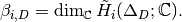
Example. Consider the graph:
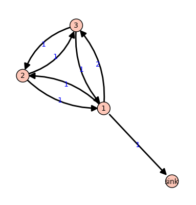
All edges have weight  except for the edge from vertex 1 to vertex 3,
which has weight
except for the edge from vertex 1 to vertex 3,
which has weight  . If we let
  with the indicated number of
grains of sand on vertices 1, 2, and 3, respectively, then only vertex 1,
whose out-degree is 4, is unstable. Firing vertex 1 gives a new
configuration
with the indicated number of
grains of sand on vertices 1, 2, and 3, respectively, then only vertex 1,
whose out-degree is 4, is unstable. Firing vertex 1 gives a new
configuration  . Here,
  grains have left vertex 1. One of
these has gone to the sink vertex (and forgotten), one has gone to vertex 1,
and two have gone to vertex 2, since the edge from 1 to 2 has weight 2.
Vertex 3 in the new configuration is now unstable. The Sage code for this
example looks like this:
grains have left vertex 1. One of
these has gone to the sink vertex (and forgotten), one has gone to vertex 1,
and two have gone to vertex 2, since the edge from 1 to 2 has weight 2.
Vertex 3 in the new configuration is now unstable. The Sage code for this
example looks like this:
Create the sandpile:

    sage: g = {'sink':{},
               1:{'sink':1, 2:1, 3:2},
               2:{1:1, 3:1},
               3:{1:1, 2:1}}
    sage: S = Sandpile(g, 'sink')
    sage: S.show(edge_labels=true)  # to display the graph

Create the configuration:

    sage: c = SandpileConfig(S, {1:5, 2:0, 3:1})
    sage: S.out_degree()
    {1: 4, 2: 2, 3: 2, 'sink': 0}

Fire vertex one:

   sage: c.fire_vertex(1)
   {1: 1, 2: 1, 3: 3}

The configuration is unchanged:

    sage: c
    {1: 5, 2: 0, 3: 1}

Repeatedly fire vertices until the configuration becomes stable:

    sage: c.stabilize()
    {1: 2, 2: 1, 3: 1}

Alternatives:

    sage: ~c             # shorthand for c.stabilize()
    {1: 2, 2: 1, 3: 1}
    sage: c.stabilize(with_firing_vector=true)
    [{1: 2, 2: 1, 3: 1}, {1: 2, 2: 2, 3: 3}]
Since vertex 3 has become unstable after firing vertex 1, it can be fired,
which causes vertex 2 to become unstable, etc. Repeated firings eventually
lead to a stable configuration. The last line of the Sage code, above, is a
list, the first element of which is the resulting stable configuration,
 . The second component records how many times each vertex fired in
the stabilization.
. The second component records how many times each vertex fired in
the stabilization.
Since the sink is accessible from each nonsink vertex and never fires, every configuration will stabilize after a finite number of vertex-firings. It is not obvious, but the resulting stabilization is independent of the order in which unstable vertices are fired. Thus, each configuration stabilizes to a unique stable configuration.
Fix an order on the vertices of . The Laplacian of is

where  is the diagonal matrix of out-degrees of the vertices and
  is the
adjacency matrix whose
is the
adjacency matrix whose  -th entry is the weight of the edge from vertex
 to vertex
  , which we take to be
  if there is no edge. The reduced
Laplacian,
if there is no edge. The reduced
Laplacian,  , is the submatrix of the Laplacian formed by removing
the row and column corresponding to the sink vertex. Firing a vertex of a
configuration is the same as subtracting the corresponding row of the reduced
Laplacian.
, is the submatrix of the Laplacian formed by removing
the row and column corresponding to the sink vertex. Firing a vertex of a
configuration is the same as subtracting the corresponding row of the reduced
Laplacian.
Example. (Continued.)
    sage: S.vertices()  # here is the ordering of the vertices
    [1, 2, 3, 'sink']
    sage: S.laplacian()
    [ 4 -1 -2 -1]
    [-1  2 -1  0]
    [-1 -1  2  0]
    [ 0  0  0  0]
    sage: S.reduced_laplacian()
    [ 4 -1 -2]
    [-1  2 -1]
    [-1 -1  2]

The configuration we considered previously:

    sage: c = SandpileConfig(S, [5,0,1])
    sage: c
    {1: 5, 2: 0, 3: 1}

Firing vertex 1 is the same as subtracting the
corresponding row from the reduced Laplacian:

    sage: c.fire_vertex(1).values()
    [1, 1, 3]
    sage: S.reduced_laplacian()[0]
    (4, -1, -2)
    sage: vector([5,0,1]) - vector([4,-1,-2])
    (1, 1, 3)
Imagine an experiment in which grains of sand are dropped one-at-a-time onto a graph, pausing to allow the configuration to stabilize between drops. Some configurations will only be seen once in this process. For example, for most graphs, once sand is dropped on the graph, no addition of sand+stabilization will result in a graph empty of sand. Other configurations—the so-called recurrent configurations—will be seen infinitely often as the process is repeated indefinitely.
To be precise, a configuration is recurrent if (i) it is stable, and (ii)
given any configuration  , there is a configuration
  such that
 , the stabilization of
  .
.
The maximal-stable configuration, denoted  is defined by
 for all nonsink vertices . It is clear that is recurrent. Further, it is not hard to see that a configuration is recurrent if and only if it has the form
  for some configuration .
Example. (Continued.)
    sage: S.recurrents(verbose=false)
    [[3, 1, 1], [2, 1, 1], [3, 1, 0]]
    sage: c = SandpileConfig(S, [2,1,1])
    sage: c
    {1: 2, 2: 1, 3: 1}
    sage: S.is_recurrent(c)
    True
    sage: S.max_stable()
    {1: 3, 2: 1, 3: 1}

Adding any configuration to the max-stable configuration and stabilizing
yields a recurrent configuration.

    sage: x = SandpileConfig(S, [1,0,0])
    sage: x + S.max_stable()
    {1: 4, 2: 1, 3: 1}

Use & to add and stabilize:

    sage: c = x & S.max_stable()
    sage: c
    {1: 3, 2: 1, 3: 0}
    sage: c.is_recurrent()
    True

Note the various ways of performing addition + stabilization:

    sage: m = S.max_stable()
    sage: (x + m).stabilize() == ~(x + m)
    True
    sage: (x + m).stabilize() == x & m
    True
A burning configuration is a nonnegative integer-linear combination of the
rows of the reduced Laplacian matrix having nonnegative entries and such that
every vertex has a path from some vertex in its support. The corresponding
burning script gives the integer-linear combination needed to obtain the
burning configuration. So if is the burning configuration,  is its
script, and is the reduced Laplacian, then
is its
script, and is the reduced Laplacian, then  .
The minimal burning configuration is the one with the minimal script (its
components are no larger than the components of any other script for a burning
configuration).
.
The minimal burning configuration is the one with the minimal script (its
components are no larger than the components of any other script for a burning
configuration).
The following are equivalent for a configuration with burning
configuration having script :
stabilizes to
- the firing vector for the stabilization of
The burning configuration and script are computed using a modified version of Speer’s script algorithm. This is a generalization to directed multigraphs of Dhar’s burning algorithm.
Example.
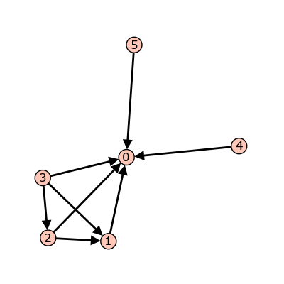
sage: g = {0:{},1:{0:1,3:1,4:1},2:{0:1,3:1,5:1},
           3:{2:1,5:1},4:{1:1,3:1},5:{2:1,3:1}}
sage: G = Sandpile(g,0)
sage: G.burning_config()
{1: 2, 2: 0, 3: 1, 4: 1, 5: 0}
sage: G.burning_config().values()
[2, 0, 1, 1, 0]
sage: G.burning_script()
{1: 1, 2: 3, 3: 5, 4: 1, 5: 4}
sage: G.burning_script().values()
[1, 3, 5, 1, 4]
sage: matrix(G.burning_script().values())*G.reduced_laplacian()
[2 0 1 1 0]
The collection of stable configurations forms a commutative monoid with addition defined as ordinary addition followed by stabilization. The identity element is the all-zero configuration. This monoid is a group exactly when the underlying graph is a DAG (directed acyclic graph).
The recurrent elements form a submonoid which turns out to be a group. This
group is called the sandpile group for , denoted
 . Its identity element is usually not the all-zero
configuration (again, only in the case that is a DAG). So finding the
identity element is an interesting problem.
. Its identity element is usually not the all-zero
configuration (again, only in the case that is a DAG). So finding the
identity element is an interesting problem.
Let  and fix an ordering of the nonsink vertices. Let
 denote the column-span of
 , the transpose of the reduced Laplacian. It is a theorem that
Thus, the number of elements of the sandpile group is  , which
by the matrix-tree theorem is the number of weighted trees directed into the
sink.
, which
by the matrix-tree theorem is the number of weighted trees directed into the
sink.
Example. (Continued.)
    sage: S.group_order()
    3
    sage: S.invariant_factors()
    [1, 1, 3]
    sage: S.reduced_laplacian().dense_matrix().smith_form()
    ([1 0 0]
    [0 1 0]
    [0 0 3],
     [ 0  0  1]
    [ 1  0  0]
    [ 0  1 -1],
     [3 1 4]
    [4 1 6]
    [4 1 5])

Adding the identity to any recurrent configuration and stabilizing yields
the same recurrent configuration:

    sage: S.identity()
    {1: 3, 2: 1, 3: 0}
    sage: i = S.identity()
    sage: m = S.max_stable()
    sage: i & m == m
    True
The sandpile model was introduced by Bak, Tang, and Wiesenfeld in the paper,
Self-organized criticality: an explanation of 1/ƒ noise [BTW]. The term
self-organized criticality has no precise definition, but can be
loosely taken to describe a system that naturally evolves to a state that is
barely stable and such that the instabilities are described by a power law.
In practice, self-organized criticality is often taken to mean like the
sandpile model on a grid-graph. The grid graph is just a grid with an extra
sink vertex. The vertices on the interior of each side have one edge to the
sink, and the corner vertices have an edge of weight . Thus, every nonsink
vertex has out-degree .
Imagine repeatedly dropping grains of sand on and empty grid graph, allowing the sandpile to stabilize in between. At first there is little activity, but as time goes on, the size and extent of the avalanche caused by a single grain of sand becomes hard to predict. Computer experiments—I do not think there is a proof, yet—indicate that the distribution of avalanche sizes obeys a power law with exponent -1. In the example below, the size of an avalanche is taken to be the sum of the number of times each vertex fires.
Example.
Distribution of avalanche sizes:

    sage: S = grid_sandpile(10,10)
    sage: m = S.max_stable()
    sage: a = []
    sage: for i in range(10000):
    ...       m = m.add_random()
    ...       m, f = m.stabilize(true)
    ...       a.append(sum(f.values()))
    ...

    sage: p = list_plot([[log(i+1),log(a.count(i))] for i in [0..max(a)] if a.count(i)])
    sage: p.axes_labels(['log(N)','log(D(N))'])
    sage: p
Distribution of avalanche sizes
Note: In the above code, m.stabilize(true) returns a list consisting of the stabilized configuration and the firing vector. (Omitting true would give just the stabilized configuration.)
A reference for this section is Riemann-Roch and Abel-Jacobi theory on a finite graph [BN].
A divisor on is an element of the free abelian group on its
vertices, including the sink. Suppose, as above, that the  vertices of
have been ordered, and that
vertices of
have been ordered, and that  is the column span of the
transpose of the Laplacian. A divisor is then identified with an element
is the column span of the
transpose of the Laplacian. A divisor is then identified with an element
 and two divisors are linearly equivalent if they
differ by an element of . A divisor
and two divisors are linearly equivalent if they
differ by an element of . A divisor  is effective, written
 , if
, if  for each
  , i.e., if
  .
The degree of a divisor, , is
.
The degree of a divisor, , is  . The
divisors of degree zero modulo linear equivalence form the Picard group, or
Jacobian of the graph. For an undirected graph, the Picard group is
isomorphic to the sandpile group.
. The
divisors of degree zero modulo linear equivalence form the Picard group, or
Jacobian of the graph. For an undirected graph, the Picard group is
isomorphic to the sandpile group.
The complete linear system for a divisor , denoted  , is the
collection of effective divisors linearly equivalent to
, is the
collection of effective divisors linearly equivalent to 
To describe the Riemann-Roch theorem in this context, suppose that is
an undirected, unweighted graph. The dimension,  of the linear system
is
of the linear system
is  if
if  and otherwise is the greatest integer such
that
and otherwise is the greatest integer such
that  for all effective divisors of degree . Define the
canonical divisor by
for all effective divisors of degree . Define the
canonical divisor by 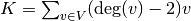 and the genus by
 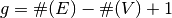 . The Riemann-Roch theorem says that for any divisor ,

Example. (Some of the following calculations require the installation of 4ti2.)
The sandpile on the complete graph on 5 vertices:

    sage: G = complete_sandpile(5)

The genus (num_edges method counts each undirected edge twice):

    sage: g = G.num_edges()/2 - G.num_verts() + 1

A divisor on the graph:

    sage: D = SandpileDivisor(G, [1,2,2,0,2])

Verify the Riemann-Roch theorem:

    sage: K = G.canonical_divisor()
    sage: D.r_of_D() - (K - D).r_of_D() == D.deg() + 1 - g
    True

The effective divisors linearly equivalent to D:

    sage: [E.values() for E in D.effective_div()]
    [[0, 1, 1, 4, 1], [4, 0, 0, 3, 0], [1, 2, 2, 0, 2]]

The nonspecial divisors up to linear equivalence (divisors of degree
g-1 with empty linear systems)

    sage: N = G.nonspecial_divisors()
    sage: [E.values() for E in N[:5]]   # the first few

    [[-1, 2, 1, 3, 0],
     [-1, 0, 3, 1, 2],
     [-1, 2, 0, 3, 1],
     [-1, 3, 1, 2, 0],
     [-1, 2, 0, 1, 3]]
    sage: len(N)
    24
    sage: len(N) == G.h_vector()[-1]
    True
Fix a divisor . There are at least two natural graphs associated with
linear system associated with . First, consider the directed graph with
vertex set and with an edge from vertex to vertex  if is
attained from by firing a single unstable vertex.
if is
attained from by firing a single unstable vertex.
sage: S = Sandpile(graphs.CycleGraph(6),0)
sage: D = SandpileDivisor(S, [1,1,1,1,2,0])
sage: D.is_alive()
True
sage: eff = D.effective_div()
sage:
firing_graph(S,eff).show3d(edge_size=.005,vertex_size=0.01,iterations=500)
Complete linear system for (1,1,1,1,2,0) on  : single firings
The second graph has the same set of vertices but with an edge from to
if is obtained from by firing all unstable vertices of .
sage: S = Sandpile(graphs.CycleGraph(6),0)
sage: D = SandpileDivisor(S, [1,1,1,1,2,0])
sage: eff = D.effective_div()
sage: parallel_firing_graph(S,eff).show3d(edge_size=.005,vertex_size=0.01,iterations=500)
Complete linear system for (1,1,1,1,2,0) on : parallel firings
Note that in each of the examples, above, starting at any divisor in the linear system and following edges, one is eventually led into a cycle of length 6 (cycling the divisor (1,1,1,1,2,0)). Thus, D.alive() returns True. In Sage, one would be able to rotate the above figures to get a better idea of the structure.
Let , and fix an ordering on the nonsink vertices of . let
 denote the column-span of
, the transpose of the reduced Laplacian. Label vertex with the
indeterminate
denote the column-span of
, the transpose of the reduced Laplacian. Label vertex with the
indeterminate  , and let
 ![\mathbb{C}[\Gamma_s] = \mathbb{C}[x_1,\dots,x_n]](_images/math/e1ef1ba99ea450324dab0463f91ec0e0ad5e59cc.png) .
(Here, denotes the sink vertex of .) The sandpile ideal or
toppling ideal, first studied by Cori, Rossin, and Salvy [CRS] for undirected graphs, is the lattice ideal for
.
(Here, denotes the sink vertex of .) The sandpile ideal or
toppling ideal, first studied by Cori, Rossin, and Salvy [CRS] for undirected graphs, is the lattice ideal for  :
:
![I = I(\Gamma_s) := \{x^u-x^v: u-v\in
\tilde{\mathcal{L}}\}\subset\mathbb{C}[\Gamma_s],](_images/math/fe585a5c73620931ddb2217cd4e222a78eaca500.png)
where  for
for  .
.
For each  define
  where
where
 and
and  so that
  .
Then, for each
.
Then, for each  , define
  . It then turns out that

where  is the -th standard basis vector and is any burning
configuration.
is the -th standard basis vector and is any burning
configuration.
The affine coordinate ring, ![\mathbb{C}[\Gamma_s]/I,](_images/math/c86f192525ebd188ad7eba9f1677c8078a919e95.png) is isomorphic to the group
algebra of the sandpile group,
is isomorphic to the group
algebra of the sandpile group, ![\mathbb{C}[\mathcal{S}(\Gamma)].](_images/math/56f2228438171b93edb6630402ebc5382f18caf9.png)
The standard term-ordering on ![\mathbb{C}[\Gamma_s]](_images/math/3137ebe0914960c96f1bf4ced19fd81ae0d8b321.png) is graded reverse
lexigraphical order with
is graded reverse
lexigraphical order with  if vertex
  is further from the sink than
vertex
is further from the sink than
vertex  . (There are choices to be made for vertices equidistant from the
sink). If
. (There are choices to be made for vertices equidistant from the
sink). If  is the script for a burning configuration (not
necessarily minimal), then
is the script for a burning configuration (not
necessarily minimal), then
is a Groebner basis for  .
.
Now let ![\mathbb{C}[\Gamma]=\mathbb{C}[x_0,x_1,\dots,x_n]](_images/math/89b6b44feba8cbf1687365cfbcaff81331aff2f4.png) , where
, where  corresponds to the sink vertex. The homogeneous sandpile ideal, denoted
 , is obtaining by homogenizing with respect to . Let
  be the
(full) Laplacian, and
be the
(full) Laplacian, and  be the column span of
its transpose,
be the column span of
its transpose,  Then is the lattice ideal for :
![I^h = I^h(\Gamma) := \{x^u-x^v: u-v \in\mathcal{L}\}\subset\mathbb{C}[\Gamma].](_images/math/efc956d162e507dd37203fc62f377ccd0e66e311.png)
This ideal can be calculated by saturating the ideal
with respect to the product of the indeterminates:  (extending
the
(extending
the  operator in the obvious way). A Groebner basis with respect to the
degree lexicographic order describe above (with the smallest vertex), is
obtained by homogenizing each element of the Groebner basis for the
non-homogeneous sandpile ideal with respect to
operator in the obvious way). A Groebner basis with respect to the
degree lexicographic order describe above (with the smallest vertex), is
obtained by homogenizing each element of the Groebner basis for the
non-homogeneous sandpile ideal with respect to 
Example.
    sage: g = {0:{},1:{0:1,3:1,4:1},2:{0:1,3:1,5:1},
               3:{2:1,5:1},4:{1:1,3:1},5:{2:1,3:1}}
    sage: S = Sandpile(g, 0)
    sage: S.ring()
    Multivariate Polynomial Ring in x5, x4, x3, x2, x1, x0 over Rational Field

The homogeneous sandpile ideal:

    sage: S.ideal()
    Ideal (x2 - x0, x3^2 - x5*x0, x5*x3 - x0^2, x4^2 - x3*x1, x5^2 - x3*x0,
    x1^3 - x4*x3*x0, x4*x1^2 - x5*x0^2) of Multivariate Polynomial Ring
    in x5, x4, x3, x2, x1, x0 over Rational Field

The generators of the ideal:

    sage: S.ideal(true)
    [x2 - x0,
     x3^2 - x5*x0,
     x5*x3 - x0^2,
     x4^2 - x3*x1,
     x5^2 - x3*x0,
     x1^3 - x4*x3*x0,
     x4*x1^2 - x5*x0^2]

Its resolution:

    sage: S.resolution()
    'R <-- R^7 <-- R^19 <-- R^25 <-- R^16 <-- R^4'

and Betti table:

    sage: S.betti()
               0     1     2     3     4     5
    ------------------------------------------
        0:     1     1     -     -     -     -
        1:     -     4     6     2     -     -
        2:     -     2     7     7     2     -
        3:     -     -     6    16    14     4
    ------------------------------------------
    total:     1     7    19    25    16     4

The Hilbert function:

    sage: S.hilbert_function()
    [1, 5, 11, 15]

and its first differences (which counts the number of superstable
configurations in each degree):

    sage: S.h_vector()
    [1, 4, 6, 4]
    sage: x = [sum(i) for i in S.superstables(False)]
    sage: sorted(x)
    [0, 1, 1, 1, 1, 2, 2, 2, 2, 2, 2, 3, 3, 3, 3]

The degree in which the Hilbert function equals the Hilbert polynomial, the
latter always being a constant in the case of a sandpile ideal:

    sage: S.postulation()
    3
The zero set for the sandpile ideal is

the set of simultaneous zeros of the polynomials in  Letting
  denote
the unit circle in the complex plane,
denote
the unit circle in the complex plane,  is a finite
subgroup of
is a finite
subgroup of  , isomorphic to the
sandpile group. The zero set is actually linearly isomorphic to a faithful representation of the sandpile group on
, isomorphic to the
sandpile group. The zero set is actually linearly isomorphic to a faithful representation of the sandpile group on 
Example. (Continued.)
     sage: S = Sandpile({0: {}, 1: {2: 2}, 2: {0: 4, 1: 1}}, 0)
     sage: S.ideal().gens()
     [x1^2 - x2^2, x1*x2^3 - x0^4, x2^5 - x1*x0^4]

Approximation to the zero set (setting ``x_0 = 1``):

     sage: S.solve()
     [[0.707107*I - 0.707107, 0.707107 - 0.707107*I],
      [-0.707107*I - 0.707107, 0.707107*I + 0.707107],
      [-1*I, -1*I],
      [I, I],
      [0.707107*I + 0.707107, -0.707107*I - 0.707107],
      [0.707107 - 0.707107*I, 0.707107*I - 0.707107],
      [1, 1],
      [-1, -1]]
     sage: len(_) == S.group_order()
     True

 The zeros are generated as a group by a single vector:

     sage: S.points()
     [[e^(1/4*I*pi), e^(-3/4*I*pi)]]
The homogeneous sandpile ideal, , has a free resolution graded by the
divisors on modulo linear equivalence. (See the section on
Discrete Riemann Surfaces for the language of
divisors and linear equivalence.) Let
![S=\mathbb{C}[\Gamma]=\mathbb{C}[x_0,\dots,x_n]](_images/math/2cb933567163075ccbd51b470c14654e26fc0b71.png) , as above, and let
, as above, and let
 denote the group of divisors modulo rational equivalence. Then
 is graded by by letting
  for
each monomial
for
each monomial  . The minimal free resolution of has the form

where the  are the Betti numbers for .
For each divisor class  , define a simplicial complex,

The Betti number equals the dimension over  of the
-th reduced homology group of
of the
-th reduced homology group of  :
:
        sage: S = Sandpile({0:{},1:{0: 1, 2: 1, 3: 4},2:{3: 5},3:{1: 1, 2: 1}},0)

Representatives of all divisor classes with nontrivial homology:

    sage: p = S.betti_complexes()
    sage: p[0]
    [{0: -8, 1: 5, 2: 4, 3: 1},
     Simplicial complex with vertex set (0, 1, 2, 3) and facets {(1, 2), (3,)}]

The homology associated with the first divisor in the list:

    sage: D = p[0][0]
    sage: D.effective_div()
    [{0: 0, 1: 1, 2: 1, 3: 0}, {0: 0, 1: 0, 2: 0, 3: 2}]
    sage: [E.support() for E in D.effective_div()]
    [[1, 2], [3]]
    sage: D.Dcomplex()
    Simplicial complex with vertex set (0, 1, 2, 3) and facets {(1, 2), (3,)}
    sage: D.Dcomplex().homology()
    {0: Z, 1: 0}


The minimal free resolution:

    sage: S.resolution()
    'R <-- R^5 <-- R^5 <-- R^1'
    sage: S.betti()
               0     1     2     3
    ------------------------------
        0:     1     -     -     -
        1:     -     5     5     -
        2:     -     -     -     1
    ------------------------------
    total:     1     5     5     1
    sage: len(p)
    11

The degrees and ranks of the homology groups for each element of the list p
(compare with the Betti table, above):

    sage: [[sum(d[0].values()),d[1].betti()] for d in p]

    [[2, {0: 1, 1: 0}],
     [3, {0: 0, 1: 1, 2: 0}],
     [2, {0: 1, 1: 0}],
     [3, {0: 0, 1: 1, 2: 0}],
     [2, {0: 1, 1: 0}],
     [3, {0: 0, 1: 1, 2: 0}],
     [2, {0: 1, 1: 0}],
     [3, {0: 0, 1: 1}],
     [2, {0: 1, 1: 0}],
     [3, {0: 0, 1: 1, 2: 0}],
     [5, {0: 0, 1: 0, 2: 1}]]
NOTE: in the previous section note that the resolution always has length n since the ideal is Cohen-Macaulay.
To do.
To do.
Warning
The methods for computing linear systems of divisors and their corresponding simplicial complexes require the installation of 4ti2.
To install 4ti2:
sage -i 4ti2.p0
There are three main classes for sandpile structures in Sage: Sandpile, SandpileConfig, and SandpileDivisor. Initialization for Sandpile has the form
sage: S = Sandpile(graph, sink)
where graph represents a graph and sink is the key for the sink vertex. There are four possible forms for graph:
sage: g = {0: {}, 1: {0: 1, 3: 1, 4: 1}, 2: {0: 1, 3: 1, 5: 1},
           3: {2: 1, 5: 1}, 4: {1: 1, 3: 1}, 5: {2: 1, 3: 1}}
Graph from dictionary of dictionaries.
Each key is the name of a vertex. Next to each vertex name is a dictionary
consisting of pairs: vertex: weight. Each pair represents a directed edge
emanating from and ending at vertex having (non-negative integer) weight
equal to weight. Loops are allowed. In the example above, all of the weights are 1.
sage: g = {0: [], 1: [0, 3, 4], 2: [0, 3, 5],
           3: [2, 5], 4: [1, 3], 5: [2, 3]}
This is a short-hand when all of the edge-weights are equal to 1. The above example is for the same displayed graph.
sage: g = graphs.CycleGraph(5)
sage: S = Sandpile(g, 0)
sage: type(g)
<class 'sage.graphs.graph.Graph'>
To see the types of built-in graphs, type graphs., including the period, and hit TAB.
sage: S = Sandpile(digraphs.RandomDirectedGNC(6), 0)
sage: S.show()
A random graph.
See ../reference/sage/graphs/graph_generators.html for more information on the Sage graph library and graph constructors.
Each of these four formats is preprocessed by the Sandpile class so that, internally, the graph is represented by the dictionary of dictionaries format first presented. This internal format is returned by dict():
sage: S  = Sandpile({0:[], 1:[0, 3, 4], 2:[0, 3, 5],
                     3: [2, 5], 4: [1, 3], 5: [2, 3]},0)
sage: S.dict()

{0: {},
 1: {0: 1, 3: 1, 4: 1},
 2: {0: 1, 3: 1, 5: 1},
 3: {2: 1, 5: 1},
 4: {1: 1, 3: 1},
 5: {2: 1, 3: 1}}
Note
The user is responsible for assuring that each vertex has a directed path into the designated sink. If the sink has out-edges, these will be ignored for the purposes of sandpile calculations (but not calculations on divisors).
Code for checking whether a given vertex is a sink:
sage:  S  = Sandpile({0:[], 1:[0, 3, 4], 2:[0, 3, 5],
                         3: [2, 5], 4: [1, 3], 5: [2, 3]},0)
sage: [S.distance(v,0) for v in S.vertices()] # 0 is a sink
[0, 1, 1, 2, 2, 2]
sage: [S.distance(v,1) for v in S.vertices()] # 1 is not a sink
[+Infinity, 0, +Infinity, +Infinity, 1, +Infinity]
Here are summaries of Sandpile, SandpileConfig, and SandpileDivisor methods (functions). Each summary is followed by a list of complete descriptions of the methods. There are many more methods available for a Sandpile, e.g., those inherited from the class DiGraph. To see them all, enter
sage: dir(Sandpile)
or type Sandpile., including the period, and hit TAB.
Summary of methods.
Complete descriptions of Sandpile methods.
—
all_k_config(k)
The configuration with all values set to k.
INPUT:
k - integer
OUTPUT:
SandpileConfig
EXAMPLES:
sage: S = sandlib('generic')
sage: S.all_k_config(7)
{1: 7, 2: 7, 3: 7, 4: 7, 5: 7}
—
all_k_div(k)
The divisor with all values set to k.
INPUT:
k - integer
OUTPUT:
SandpileDivisor
EXAMPLES:
sage: S = sandlib('generic')
sage: S.all_k_div(7)
{0: 7, 1: 7, 2: 7, 3: 7, 4: 7, 5: 7}
—
betti(verbose=True)
Computes the Betti table for the homogeneous sandpile ideal. If verbose is True, it prints the standard Betti table, otherwise, it returns a less formated table.
INPUT:
verbose (optional) - boolean
OUTPUT:
Betti numbers for the sandpile
EXAMPLES:
sage: S = sandlib('generic')
sage: S.betti() # long time
           0     1     2     3     4     5
------------------------------------------
    0:     1     1     -     -     -     -
    1:     -     4     6     2     -     -
    2:     -     2     7     7     2     -
    3:     -     -     6    16    14     4
------------------------------------------
total:     1     7    19    25    16     4
sage: S.betti(False) # long time
[1, 7, 19, 25, 16, 4]
—
betti_complexes()
A list of all the divisors with nonempty linear systems whose corresponding simplicial complexes have nonzero homology in some dimension. Each such divisor is returned with its corresponding simplicial complex.
INPUT:
None
OUTPUT:
list (of pairs [divisors, corresponding simplicial complex])
EXAMPLES:
sage: S = Sandpile({0:{},1:{0: 1, 2: 1, 3: 4},2:{3: 5},3:{1: 1, 2: 1}},0)
sage: p = S.betti_complexes() # optional - 4ti2
sage: p[0] # optional - 4ti2
[{0: -8, 1: 5, 2: 4, 3: 1},
 Simplicial complex with vertex set (0, 1, 2, 3) and facets {(1, 2), (3,)}]
sage: S.resolution()
'R^1 <-- R^5 <-- R^5 <-- R^1'
sage: S.betti()
           0     1     2     3
------------------------------
    0:     1     -     -     -
    1:     -     5     5     -
    2:     -     -     -     1
------------------------------
total:     1     5     5     1
sage: len(p) # optional - 4ti2
11
sage: p[0][1].homology() # optional - 4ti2
{0: Z, 1: 0}
sage: p[-1][1].homology() # optional - 4ti2
{0: 0, 1: 0, 2: Z}
—
burning_config()
A minimal burning configuration.
INPUT:
None
OUTPUT:
dict (configuration)
EXAMPLES:
sage: g = {0:{},1:{0:1,3:1,4:1},2:{0:1,3:1,5:1},\
           3:{2:1,5:1},4:{1:1,3:1},5:{2:1,3:1}}
sage: S = Sandpile(g,0)
sage: S.burning_config()
{1: 2, 2: 0, 3: 1, 4: 1, 5: 0}
sage: S.burning_config().values()
[2, 0, 1, 1, 0]
sage: S.burning_script()
{1: 1, 2: 3, 3: 5, 4: 1, 5: 4}
sage: script = S.burning_script().values()
sage: script
[1, 3, 5, 1, 4]
sage: matrix(script)*S.reduced_laplacian()
[2 0 1 1 0]
NOTES:
The burning configuration and script are computed using a modified version of Speer’s script algorithm. This is a generalization to directed multigraphs of Dhar’s burning algorithm.
A burning configuration is a nonnegative integer-linear combination of the rows of the reduced Laplacian matrix having nonnegative entries and such that every vertex has a path from some vertex in its support. The corresponding burning script gives the integer-linear combination needed to obtain the burning configuration. So if b is the burning configuration, sigma is its script, and tilde{L} is the reduced Laplacian, then sigma * tilde{L} = b. The minimal burning configuration is the one with the minimal script (its components are no larger than the components of any other script for a burning configuration).
The following are equivalent for a configuration c with burning configuration b having script sigma:
- c is recurrent;
- c+b stabilizes to c;
- the firing vector for the stabilization of c+b is sigma.
—
burning_script()
A script for the minimal burning configuration.
INPUT:
None
OUTPUT:
dict
EXAMPLES:
sage: g = {0:{},1:{0:1,3:1,4:1},2:{0:1,3:1,5:1},\
3:{2:1,5:1},4:{1:1,3:1},5:{2:1,3:1}}
sage: S = Sandpile(g,0)
sage: S.burning_config()
{1: 2, 2: 0, 3: 1, 4: 1, 5: 0}
sage: S.burning_config().values()
[2, 0, 1, 1, 0]
sage: S.burning_script()
{1: 1, 2: 3, 3: 5, 4: 1, 5: 4}
sage: script = S.burning_script().values()
sage: script
[1, 3, 5, 1, 4]
sage: matrix(script)*S.reduced_laplacian()
[2 0 1 1 0]
NOTES:
The burning configuration and script are computed using a modified version of Speer’s script algorithm. This is a generalization to directed multigraphs of Dhar’s burning algorithm.
A burning configuration is a nonnegative integer-linear combination of the rows of the reduced Laplacian matrix having nonnegative entries and such that every vertex has a path from some vertex in its support. The corresponding burning script gives the integer-linear combination needed to obtain the burning configuration. So if b is the burning configuration, s is its script, and L_{mathrm{red}} is the reduced Laplacian, then s * L_{mathrm{red}}= b. The minimal burning configuration is the one with the minimal script (its components are no larger than the components of any other script for a burning configuration).
The following are equivalent for a configuration c with burning configuration b having script s:
- c is recurrent;
- c+b stabilizes to c;
- the firing vector for the stabilization of c+b is s.
—
canonical_divisor()
The canonical divisor: the divisor deg(v)-2 grains of sand on each vertex. Only for undirected graphs.
INPUT:
None
OUTPUT:
SandpileDivisor
EXAMPLES:
sage: S = complete_sandpile(4)
sage: S.canonical_divisor()
{0: 1, 1: 1, 2: 1, 3: 1}
—
dict()
A dictionary of dictionaries representing a directed graph.
INPUT:
None
OUTPUT:
dict
EXAMPLES:
sage: G = sandlib('generic')
sage: G.dict()
{0: {},
 1: {0: 1, 3: 1, 4: 1},
 2: {0: 1, 3: 1, 5: 1},
 3: {2: 1, 5: 1},
 4: {1: 1, 3: 1},
 5: {2: 1, 3: 1}}
sage: G.sink()
0
—
groebner()
A Groebner basis for the homogeneous sandpile ideal with respect to the standard sandpile ordering (see ring).
INPUT:
None
OUTPUT:
Groebner basis
EXAMPLES:
sage: S = sandlib('generic')
sage: S.groebner()
[x4*x1^2 - x5*x0^2, x1^3 - x4*x3*x0, x5^2 - x3*x0, x4^2 - x3*x1, x5*x3 - x0^2,
x3^2 - x5*x0, x2 - x0]
—
group_order()
The size of the sandpile group.
INPUT:
None
OUTPUT:
int
EXAMPLES:
sage: S = sandlib('generic')
sage: S.group_order()
15
—
h_vector()
The first differences of the Hilbert function of the homogeneous sandpile ideal. It lists the number of superstable configurations in each degree.
INPUT:
None
OUTPUT:
list of nonnegative integers
EXAMPLES:
sage: S = sandlib('generic')
sage: S.hilbert_function()
[1, 5, 11, 15]
sage: S.h_vector()
[1, 4, 6, 4]
—
hilbert_function()
The Hilbert function of the homogeneous sandpile ideal.
INPUT:
None
OUTPUT:
list of nonnegative integers
EXAMPLES:
sage: S = sandlib('generic')
sage: S.hilbert_function()
[1, 5, 11, 15]
—
ideal(gens=False)
The saturated, homogeneous sandpile ideal (or its generators if gens=True).
INPUT:
verbose (optional) - boolean
OUTPUT:
ideal or, optionally, the generators of an ideal
EXAMPLES:
sage: S = sandlib('generic')
sage: S.ideal()
Ideal (x2 - x0, x3^2 - x5*x0, x5*x3 - x0^2, x4^2 - x3*x1, x5^2 - x3*x0,
x1^3 - x4*x3*x0, x4*x1^2 - x5*x0^2) of Multivariate Polynomial Ring
in x5, x4, x3, x2, x1, x0 over Rational Field
sage: S.ideal(True)
[x2 - x0, x3^2 - x5*x0, x5*x3 - x0^2, x4^2 - x3*x1, x5^2 - x3*x0,
x1^3 - x4*x3*x0, x4*x1^2 - x5*x0^2]
sage: S.ideal().gens()  # another way to get the generators
[x2 - x0, x3^2 - x5*x0, x5*x3 - x0^2, x4^2 - x3*x1, x5^2 - x3*x0,
x1^3 - x4*x3*x0, x4*x1^2 - x5*x0^2]
—
identity()
The identity configuration.
INPUT:
None
OUTPUT:
dict (the identity configuration)
EXAMPLES:
sage: S = sandlib('generic')
sage: e = S.identity()
sage: x = e & S.max_stable()  # stable addition
sage: x
{1: 2, 2: 2, 3: 1, 4: 1, 5: 1}
sage: x == S.max_stable()
True
—
in_degree(v=None)
The in-degree of a vertex or a list of all in-degrees.
INPUT:
v - vertex name or None
OUTPUT:
integer or dict
EXAMPLES:
sage: S = sandlib('generic')
sage: S.in_degree(2)
2
sage: S.in_degree()
{0: 2, 1: 1, 2: 2, 3: 4, 4: 1, 5: 2}
—
invariant_factors()
The invariant factors of the sandpile group (a finite abelian group).
INPUT:
None
OUTPUT:
list of integers
EXAMPLES:
sage: S = sandlib('generic')
sage: S.invariant_factors()
[1, 1, 1, 1, 15]
—
is_undirected()
True if (u,v) is and edge if and only if (v,u) is an edges, each edge with the same weight.
INPUT:
None
OUTPUT:
boolean
EXAMPLES:
sage: complete_sandpile(4).is_undirected()
True
sage: sandlib('gor').is_undirected()
False
—
laplacian()
The Laplacian matrix of the graph.
INPUT:
None
OUTPUT:
matrix
EXAMPLES:
sage: G = sandlib('generic')
sage: G.laplacian()
[ 0  0  0  0  0  0]
[-1  3  0 -1 -1  0]
[-1  0  3 -1  0 -1]
[ 0  0 -1  2  0 -1]
[ 0 -1  0 -1  2  0]
[ 0  0 -1 -1  0  2]
NOTES:
The function laplacian_matrix should be avoided. It returns the indegree version of the laplacian.
—
max_stable()
The maximal stable configuration.
INPUT:
None
OUTPUT:
SandpileConfig (the maximal stable configuration)
EXAMPLES:
sage: S = sandlib('generic')
sage: S.max_stable()
{1: 2, 2: 2, 3: 1, 4: 1, 5: 1}
—
max_stable_div()
The maximal stable divisor.
INPUT:
SandpileDivisor
OUTPUT:
SandpileDivisor (the maximal stable divisor)
EXAMPLES:
sage: S = sandlib('generic')
sage: S.max_stable_div()
{0: -1, 1: 2, 2: 2, 3: 1, 4: 1, 5: 1}
sage: S.out_degree()
{0: 0, 1: 3, 2: 3, 3: 2, 4: 2, 5: 2}
—
max_superstables(verbose=True)
The maximal superstable configurations. If the underlying graph is undirected, these are the superstables of highest degree. If verbose is False, the configurations are converted to lists of integers.
INPUT:
verbose (optional) - boolean
OUTPUT:
list (of maximal superstables)
EXAMPLES:
sage: S=sandlib('riemann-roch2')
sage: S.max_superstables()
[{1: 1, 2: 1, 3: 1}, {1: 0, 2: 0, 3: 2}]
sage: S.superstables(False)
[[0, 0, 0],
 [1, 0, 1],
 [1, 0, 0],
 [0, 1, 1],
 [0, 1, 0],
 [1, 1, 0],
 [0, 0, 1],
 [1, 1, 1],
 [0, 0, 2]]
sage: S.h_vector()
[1, 3, 4, 1]
—
min_recurrents(verbose=True)
The minimal recurrent elements. If the underlying graph is undirected, these are the recurrent elements of least degree. If verbose is ``False, the configurations are converted to lists of integers.
INPUT:
verbose (optional) - boolean
OUTPUT:
list of SandpileConfig
EXAMPLES:
sage: S=sandlib('riemann-roch2')
sage: S.min_recurrents()
[{1: 0, 2: 0, 3: 1}, {1: 1, 2: 1, 3: 0}]
sage: S.min_recurrents(False)
[[0, 0, 1], [1, 1, 0]]
sage: S.recurrents(False)
[[1, 1, 2],
 [0, 1, 1],
 [0, 1, 2],
 [1, 0, 1],
 [1, 0, 2],
 [0, 0, 2],
 [1, 1, 1],
 [0, 0, 1],
 [1, 1, 0]]
sage: [i.deg() for i in S.recurrents()]
[4, 2, 3, 2, 3, 2, 3, 1, 2]
—
nonsink_vertices()
The names of the nonsink vertices.
INPUT:
None
OUTPUT:
None
EXAMPLES:
sage: S = sandlib('generic')
sage: S.nonsink_vertices()
[1, 2, 3, 4, 5]
—
nonspecial_divisors(verbose=True)
The nonspecial divisors: those divisors of degree g-1 with empty linear system. The term is only defined for undirected graphs. Here, g = |E| - |V| + 1 is the genus of the graph. If verbose is False, the divisors are converted to lists of integers.
INPUT:
verbose (optional) - boolean
OUTPUT:
list (of divisors)
EXAMPLES:
sage: S = complete_sandpile(4)
sage: ns = S.nonspecial_divisors() # optional - 4ti2
sage: D = ns[0] # optional - 4ti2
sage: D.values() # optional - 4ti2
[-1, 1, 0, 2]
sage: D.deg() # optional - 4ti2
2
sage: [i.effective_div() for i in ns] # optional - 4ti2
[[], [], [], [], [], []]
—
num_edges()
The number of edges.
EXAMPLES:
sage: G = graphs.PetersenGraph()
sage: G.size()
15
—
num_verts()
The number of vertices. Note that len(G) returns the number of vertices in G also.
EXAMPLES:
sage: G = graphs.PetersenGraph()
sage: G.order()
10

sage: G = graphs.TetrahedralGraph()
sage: len(G)
4
—
out_degree(v=None)
The out-degree of a vertex or a list of all out-degrees.
INPUT:
v (optional) - vertex name
OUTPUT:
integer or dict
EXAMPLES:
sage: S = sandlib('generic')
sage: S.out_degree(2)
3
sage: S.out_degree()
{0: 0, 1: 3, 2: 3, 3: 2, 4: 2, 5: 2}
—
points()
Generators for the multiplicative group of zeros of the sandpile ideal.
INPUT:
None
OUTPUT:
list of complex numbers
EXAMPLES:
The sandpile group in this example is cyclic, and hence there is a single generator for the group of solutions.
sage: S = sandlib('generic')
sage: S.points()
[[e^(4/5*I*pi), 1, e^(2/3*I*pi), e^(-34/15*I*pi), e^(-2/3*I*pi)]]
—
postulation()
The postulation number of the sandpile ideal. This is the largest weight of a superstable configuration of the graph.
INPUT:
None
OUTPUT:
nonnegative integer
EXAMPLES:
sage: S = sandlib('generic')
sage: S.postulation()
3
—
recurrents(verbose=True)
The list of recurrent configurations. If verbose is False, the configurations are converted to lists of integers.
INPUT:
verbose (optional) - boolean
OUTPUT:
list (of recurrent configurations)
EXAMPLES:
sage: S = sandlib('generic')
sage: S.recurrents()
[{1: 2, 2: 2, 3: 1, 4: 1, 5: 1}, {1: 2, 2: 2, 3: 0, 4: 1, 5: 1},
{1: 0, 2: 2, 3: 1, 4: 1, 5: 0}, {1: 0, 2: 2, 3: 1, 4: 1, 5: 1},
{1: 1, 2: 2, 3: 1, 4: 1, 5: 1}, {1: 1, 2: 2, 3: 0, 4: 1, 5: 1},
{1: 2, 2: 2, 3: 1, 4: 0, 5: 1}, {1: 2, 2: 2, 3: 0, 4: 0, 5: 1},
{1: 2, 2: 2, 3: 1, 4: 0, 5: 0}, {1: 1, 2: 2, 3: 1, 4: 1, 5: 0},
{1: 1, 2: 2, 3: 1, 4: 0, 5: 0}, {1: 1, 2: 2, 3: 1, 4: 0, 5: 1},
{1: 0, 2: 2, 3: 0, 4: 1, 5: 1}, {1: 2, 2: 2, 3: 1, 4: 1, 5: 0},
{1: 1, 2: 2, 3: 0, 4: 0, 5: 1}]
sage: S.recurrents(verbose=False)
[[2, 2, 1, 1, 1], [2, 2, 0, 1, 1], [0, 2, 1, 1, 0], [0, 2, 1, 1, 1],
[1, 2, 1, 1, 1], [1, 2, 0, 1, 1], [2, 2, 1, 0, 1], [2, 2, 0, 0, 1],
[2, 2, 1, 0, 0], [1, 2, 1, 1, 0], [1, 2, 1, 0, 0], [1, 2, 1, 0, 1],
[0, 2, 0, 1, 1], [2, 2, 1, 1, 0], [1, 2, 0, 0, 1]]
—
reduced_laplacian()
The reduced Laplacian matrix of the graph.
INPUT:
None
OUTPUT:
matrix
EXAMPLES:
sage: G = sandlib('generic')
sage: G.laplacian()
[ 0  0  0  0  0  0]
[-1  3  0 -1 -1  0]
[-1  0  3 -1  0 -1]
[ 0  0 -1  2  0 -1]
[ 0 -1  0 -1  2  0]
[ 0  0 -1 -1  0  2]
sage: G.reduced_laplacian()
[ 3  0 -1 -1  0]
[ 0  3 -1  0 -1]
[ 0 -1  2  0 -1]
[-1  0 -1  2  0]
[ 0 -1 -1  0  2]
NOTES:
This is the Laplacian matrix with the row and column indexed by the sink vertex removed.
—
reorder_vertices()
Create a copy of the sandpile but with the vertices ordered according to their distance from the sink, from greatest to least.
INPUT:
None
OUTPUT:
Sandpile
EXAMPLES:
sage: S = sandlib('kite')
sage: S.dict()
{0: {}, 1: {0: 1, 2: 1,
3: 1}, 2: {1: 1, 3: 1, 4: 1}, 3: {1: 1, 2: 1, 4: 1}, 4: {2: 1,
3: 1}}
sage: T = S.reorder_vertices()
sage: T.dict()
{0: {1: 1, 2: 1}, 1: {0: 1, 2: 1, 3: 1}, 2: {0: 1, 1: 1, 3: 1},
3: {1: 1, 2: 1, 4: 1}, 4: {}}
—
resolution(verbose=False)
This function computes a minimal free resolution of the homogeneous sandpile ideal. If verbose is True, then all of the mappings are returned. Otherwise, the resolution is summarized.
INPUT:
verbose (optional) - boolean
OUTPUT:
free resolution of the sandpile ideal
EXAMPLES:
sage: S = sandlib('gor')
sage: S.resolution()
'R^1 <-- R^5 <-- R^5 <-- R^1'
sage: S.resolution(True)
[
[ x1^2 - x3*x0 x3*x1 - x2*x0  x3^2 - x2*x1  x2*x3 - x0^2  x2^2 - x1*x0],
[ x3  x2   0  x0   0]  [ x2^2 - x1*x0]
[-x1 -x3  x2   0 -x0]  [-x2*x3 + x0^2]
[ x0  x1   0  x2   0]  [-x3^2 + x2*x1]
[  0   0 -x1 -x3  x2]  [x3*x1 - x2*x0]
[  0   0  x0  x1 -x3], [ x1^2 - x3*x0]
]
sage: r = S.resolution(True)
sage: r[0]*r[1]
[0 0 0 0 0]
sage: r[1]*r[2]
[0]
[0]
[0]
[0]
[0]
—
ring()
The ring containing the homogeneous sandpile ideal.
INPUT:
None
OUTPUT:
ring
EXAMPLES:
sage: S = sandlib('generic')
sage: S.ring()
Multivariate Polynomial Ring in x5, x4, x3, x2, x1, x0 over Rational Field
sage: S.ring().gens()
(x5, x4, x3, x2, x1, x0)
NOTES:
The indeterminate xi corresponds to the i-th vertex as listed my the method vertices. The term-ordering is degrevlex with indeterminates ordered according to their distance from the sink (larger indeterminates are further from the sink).
—
show(kwds)
Draws the graph.
INPUT:
kwds - arguments passed to the show method for Graph or DiGraph
OUTPUT:
None
EXAMPLES:
sage: S = sandlib('generic')
sage: S.show()
sage: S.show(graph_border=True, edge_labels=True)
—
show3d(kwds)
Draws the graph.
INPUT:
kwds - arguments passed to the show method for Graph or DiGraph
OUTPUT:
None
EXAMPLES:
sage: S = sandlib('generic')
sage: S.show3d()
—
sink()
The identifier for the sink vertex.
INPUT:
None
OUTPUT:
Object (name for the sink vertex)
EXAMPLES:
sage: G = sandlib('generic')
sage: G.sink()
0
sage: H = grid_sandpile(2,2)
sage: H.sink()
'sink'
sage: type(H.sink())
<type 'str'>
—
solve()
Approximations of the complex affine zeros of the sandpile ideal.
INPUT:
None
OUTPUT:
list of complex numbers
EXAMPLES:
sage: S = Sandpile({0: {}, 1: {2: 2}, 2: {0: 4, 1: 1}}, 0)
sage: S.solve()
[[-0.707107 + 0.707107*I, 0.707107 - 0.707107*I],
[-0.707107 - 0.707107*I, 0.707107 + 0.707107*I],
[-I, -I], [I, I], [0.707107 + 0.707107*I, -0.707107 - 0.707107*I],
[0.707107 - 0.707107*I, -0.707107 + 0.707107*I], [1, 1], [-1, -1]]
sage: len(_)
8
sage: S.group_order()
8
NOTES:
The solutions form a multiplicative group isomorphic to the sandpile group. Generators for this group are given exactly by points().
—
superstables(verbose=True)
The list of superstable configurations as dictionaries if verbose is True, otherwise as lists of integers. The superstables are also known as G-parking functions.
INPUT:
verbose (optional) - boolean
OUTPUT:
list (of superstable elements)
EXAMPLES:
sage: S = sandlib('generic')
sage: S.superstables()
[{1: 0, 2: 0, 3: 0, 4: 0, 5: 0},
 {1: 0, 2: 0, 3: 1, 4: 0, 5: 0},
 {1: 2, 2: 0, 3: 0, 4: 0, 5: 1},
 {1: 2, 2: 0, 3: 0, 4: 0, 5: 0},
 {1: 1, 2: 0, 3: 0, 4: 0, 5: 0},
 {1: 1, 2: 0, 3: 1, 4: 0, 5: 0},
 {1: 0, 2: 0, 3: 0, 4: 1, 5: 0},
 {1: 0, 2: 0, 3: 1, 4: 1, 5: 0},
 {1: 0, 2: 0, 3: 0, 4: 1, 5: 1},
 {1: 1, 2: 0, 3: 0, 4: 0, 5: 1},
 {1: 1, 2: 0, 3: 0, 4: 1, 5: 1},
 {1: 1, 2: 0, 3: 0, 4: 1, 5: 0},
 {1: 2, 2: 0, 3: 1, 4: 0, 5: 0},
 {1: 0, 2: 0, 3: 0, 4: 0, 5: 1},
 {1: 1, 2: 0, 3: 1, 4: 1, 5: 0}]
sage: S.superstables(False)
[[0, 0, 0, 0, 0],
 [0, 0, 1, 0, 0],
 [2, 0, 0, 0, 1],
 [2, 0, 0, 0, 0],
 [1, 0, 0, 0, 0],
 [1, 0, 1, 0, 0],
 [0, 0, 0, 1, 0],
 [0, 0, 1, 1, 0],
 [0, 0, 0, 1, 1],
 [1, 0, 0, 0, 1],
 [1, 0, 0, 1, 1],
 [1, 0, 0, 1, 0],
 [2, 0, 1, 0, 0],
 [0, 0, 0, 0, 1],
 [1, 0, 1, 1, 0]]
—
symmetric_recurrents(orbits)
The list of symmetric recurrent configurations.
INPUT:
orbits - list of lists partitioning the vertices
OUTPUT:
list of recurrent configurations
EXAMPLES:
sage: S = sandlib('kite')
sage: S.dict()
{0: {},
 1: {0: 1, 2: 1, 3: 1},
 2: {1: 1, 3: 1, 4: 1},
 3: {1: 1, 2: 1, 4: 1},
 4: {2: 1, 3: 1}}
sage: S.symmetric_recurrents([[1],[2,3],[4]])
[{1: 2, 2: 2, 3: 2, 4: 1}, {1: 2, 2: 2, 3: 2, 4: 0}]
sage: S.recurrents()
[{1: 2, 2: 2, 3: 2, 4: 1},
 {1: 2, 2: 2, 3: 2, 4: 0},
 {1: 2, 2: 1, 3: 2, 4: 0},
 {1: 2, 2: 2, 3: 0, 4: 1},
 {1: 2, 2: 0, 3: 2, 4: 1},
 {1: 2, 2: 2, 3: 1, 4: 0},
 {1: 2, 2: 1, 3: 2, 4: 1},
 {1: 2, 2: 2, 3: 1, 4: 1}]
NOTES:
The user is responsible for ensuring that the list of orbits comes from a group of symmetries of the underlying graph.
—
unsaturated_ideal()
The unsaturated, homogeneous sandpile ideal.
INPUT:
None
OUTPUT:
ideal
EXAMPLES:
sage: S = sandlib('generic')
sage: S.unsaturated_ideal().gens()
[x1^3 - x4*x3*x0, x2^3 - x5*x3*x0, x3^2 - x5*x2, x4^2 - x3*x1, x5^2 - x3*x2]
sage: S.ideal().gens()
[x2 - x0, x3^2 - x5*x0, x5*x3 - x0^2, x4^2 - x3*x1, x5^2 - x3*x0,
x1^3 - x4*x3*x0, x4*x1^2 - x5*x0^2]
—
version()
The version number of Sage Sandpiles.
INPUT:
None
OUTPUT:
string
EXAMPLES:
sage: S = sandlib('generic')
sage: S.version()
Sage Sandpiles Version 2.3
—
vertices(key=None, boundary_first=False)
A list of the vertices.
INPUT:
- key - default: None - a function that takes a vertex as its one argument and returns a value that can be used for comparisons in the sorting algorithm.
- boundary_first - default: False - if True, return the boundary vertices first.
OUTPUT:
The vertices of the list.
Warning: There is always an attempt to sort the list before returning the result. However, since any object may be a vertex, there is no guarantee that any two vertices will be comparable. With default objects for vertices (all integers), or when all the vertices are of the same simple type, then there should not be a problem with how the vertices will be sorted. However, if you need to guarantee a total order for the sort, use the key argument, as illustrated in the examples below.
EXAMPLES:
sage: P = graphs.PetersenGraph()
sage: P.vertices()
[0, 1, 2, 3, 4, 5, 6, 7, 8, 9]
—
zero_config()
The all-zero configuration.
INPUT:
None
OUTPUT:
SandpileConfig
EXAMPLES:
sage: S = sandlib('generic')
sage: S.zero_config()
{1: 0, 2: 0, 3: 0, 4: 0, 5: 0}
—
zero_div()
The all-zero divisor.
INPUT:
None
OUTPUT:
SandpileDivisor
EXAMPLES:
sage: S = sandlib('generic')
sage: S.zero_div()
{0: 0, 1: 0, 2: 0, 3: 0, 4: 0, 5: 0}
—
Summary of methods.
Complete descriptions of SandpileConfig methods.
—
+
Addition of configurations.
INPUT:
other - SandpileConfig
OUTPUT:
sum of self and other
EXAMPLES:
sage: S = Sandpile(graphs.CycleGraph(3), 0)
sage: c = SandpileConfig(S, [1,2])
sage: d = SandpileConfig(S, [3,2])
sage: c + d
{1: 4, 2: 4}
—
&
The stabilization of the sum.
INPUT:
other - SandpileConfig
OUTPUT:
SandpileConfig
EXAMPLES:
sage: S = Sandpile(graphs.CycleGraph(4), 0)
sage: c = SandpileConfig(S, [1,0,0])
sage: c + c  # ordinary addition
{1: 2, 2: 0, 3: 0}
sage: c & c  # add and stabilize
{1: 0, 2: 1, 3: 0}
sage: c*c  # add and find equivalent recurrent
{1: 1, 2: 1, 3: 1}
sage: ~(c + c) == c & c
True
—
>=
True if every component of self is at least that of other.
INPUT:
other - SandpileConfig
OUTPUT:
boolean
EXAMPLES:
sage: S = Sandpile(graphs.CycleGraph(3), 0)
sage: c = SandpileConfig(S, [1,2])
sage: d = SandpileConfig(S, [2,3])
sage: e = SandpileConfig(S, [2,0])
sage: c >= c
True
sage: d >= c
True
sage: c >= d
False
sage: e >= c
False
sage: c >= e
False
—
>
True if every component of self is at least that of other and the two configurations are not equal.
INPUT:
other - SandpileConfig
OUTPUT:
boolean
EXAMPLES:
sage: S = Sandpile(graphs.CycleGraph(3), 0)
sage: c = SandpileConfig(S, [1,2])
sage: d = SandpileConfig(S, [1,3])
sage: c > c
False
sage: d > c
True
sage: c > d
False
—
~
The stabilized configuration.
INPUT:
None
OUTPUT:
SandpileConfig
EXAMPLES:
sage: S = sandlib('generic')
sage: c = S.max_stable() + S.identity()
sage: ~c
{1: 2, 2: 2, 3: 1, 4: 1, 5: 1}
sage: ~c == c.stabilize()
True
—
<=
True if every component of self is at most that of other.
INPUT:
other - SandpileConfig
OUTPUT:
boolean
EXAMPLES:
sage: S = Sandpile(graphs.CycleGraph(3), 0)
sage: c = SandpileConfig(S, [1,2])
sage: d = SandpileConfig(S, [2,3])
sage: e = SandpileConfig(S, [2,0])
sage: c <= c
True
sage: c <= d
True
sage: d <= c
False
sage: c <= e
False
sage: e <= c
False
—
<
True if every component of self is at most that of other and the two configurations are not equal.
INPUT:
other - SandpileConfig
OUTPUT:
boolean
EXAMPLES:
sage: S = Sandpile(graphs.CycleGraph(3), 0)
sage: c = SandpileConfig(S, [1,2])
sage: d = SandpileConfig(S, [2,3])
sage: c < c
False
sage: c < d
True
sage: d < c
False
—
*
The recurrent element equivalent to the sum.
INPUT:
other - SandpileConfig
OUTPUT:
SandpileConfig
EXAMPLES:
sage: S = Sandpile(graphs.CycleGraph(4), 0)
sage: c = SandpileConfig(S, [1,0,0])
sage: c + c  # ordinary addition
{1: 2, 2: 0, 3: 0}
sage: c & c  # add and stabilize
{1: 0, 2: 1, 3: 0}
sage: c*c  # add and find equivalent recurrent
{1: 1, 2: 1, 3: 1}
sage: (c*c).is_recurrent()
True
sage: c*(-c) == S.identity()
True
—
^
The recurrent element equivalent to the sum of the configuration with itself k times. If k is negative, do the same for the negation of the configuration. If k is zero, return the identity of the sandpile group.
INPUT:
k - SandpileConfig
OUTPUT:
SandpileConfig
EXAMPLES:
sage: S = Sandpile(graphs.CycleGraph(4), 0)
sage: c = SandpileConfig(S, [1,0,0])
sage: c^3
{1: 1, 2: 1, 3: 0}
sage: (c + c + c) == c^3
False
sage: (c + c + c).equivalent_recurrent() == c^3
True
sage: c^(-1)
{1: 1, 2: 1, 3: 0}
sage: c^0 == S.identity()
True
—
_
The additive inverse of the configuration.
INPUT:
None
OUTPUT:
SandpileConfig
EXAMPLES:
sage: S = Sandpile(graphs.CycleGraph(3), 0)
sage: c = SandpileConfig(S, [1,2])
sage: -c
{1: -1, 2: -2}
—
-
Subtraction of configurations.
INPUT:
other - SandpileConfig
OUTPUT:
sum of self and other
EXAMPLES:
sage: S = Sandpile(graphs.CycleGraph(3), 0)
sage: c = SandpileConfig(S, [1,2])
sage: d = SandpileConfig(S, [3,2])
sage: c - d
{1: -2, 2: 0}
—
add_random()
Add one grain of sand to a random nonsink vertex.
INPUT:
None
OUTPUT:
SandpileConfig
EXAMPLES:
We compute the ‘sizes’ of the avalanches caused by adding random grains of sand to the maximal stable configuration on a grid graph. The function stabilize() returns the firing vector of the stabilization, a dictionary whose values say how many times each vertex fires in the stabilization.
sage: S = grid_sandpile(10,10)
sage: m = S.max_stable()
sage: a = []
sage: for i in range(1000):
...       m = m.add_random()
...       m, f = m.stabilize(True)
...       a.append(sum(f.values()))
...
sage: p = list_plot([[log(i+1),log(a.count(i))] for i in [0..max(a)] if a.count(i)])
sage: p.axes_labels(['log(N)','log(D(N))'])
sage: t = text("Distribution of avalanche sizes", (2,2), rgbcolor=(1,0,0))
sage: show(p+t,axes_labels=['log(N)','log(D(N))'])
—
deg()
The degree of the configuration.
INPUT:
None
OUTPUT:
integer
EXAMPLES:
sage: S = Sandpile(graphs.CycleGraph(3), 0)
sage: c = SandpileConfig(S, [1,2])
sage: c.deg()
3
—
dualize()
The difference between the maximal stable configuration and the configuration.
INPUT:
None
OUTPUT:
SandpileConfig
EXAMPLES:
sage: S = Sandpile(graphs.CycleGraph(3), 0)
sage: c = SandpileConfig(S, [1,2])
sage: S.max_stable()
{1: 1, 2: 1}
sage: c.dualize()
{1: 0, 2: -1}
sage: S.max_stable() - c == c.dualize()
True
—
equivalent_recurrent(with_firing_vector=False)
The recurrent configuration equivalent to the given configuration. Optionally returns the corresponding firing vector.
INPUT:
with_firing_vector (optional) - boolean
OUTPUT:
SandpileConfig or [SandpileConfig, firing_vector]
EXAMPLES:
sage: S = sandlib('generic')
sage: c = SandpileConfig(S, [0,0,0,0,0])
sage: c.equivalent_recurrent() == S.identity()
True
sage: x = c.equivalent_recurrent(True)
sage: r = vector([x[0][v] for v in S.nonsink_vertices()])
sage: f = vector([x[1][v] for v in S.nonsink_vertices()])
sage: cv = vector(c.values())
sage: r == cv - f*S.reduced_laplacian()
True
NOTES:
Let L be the reduced laplacian, c the initial configuration, r the returned configuration, and f the firing vector. Then r = c - f * L.
—
equivalent_superstable(with_firing_vector=False)
The equivalent superstable configuration. Optionally returns the corresponding firing vector.
INPUT:
with_firing_vector (optional) - boolean
OUTPUT:
SandpileConfig or [SandpileConfig, firing_vector]
EXAMPLES:
sage: S = sandlib('generic')
sage: m = S.max_stable()
sage: m.equivalent_superstable().is_superstable()
True
sage: x = m.equivalent_superstable(True)
sage: s = vector(x[0].values())
sage: f = vector(x[1].values())
sage: mv = vector(m.values())
sage: s == mv - f*S.reduced_laplacian()
True
NOTES:
Let L be the reduced laplacian, c the initial configuration, s the returned configuration, and f the firing vector. Then s = c - f * L.
—
fire_script(sigma)
Fire the script sigma, i.e., fire each vertex the indicated number of times.
INPUT:
sigma - SandpileConfig or (list or dict representing a SandpileConfig)
OUTPUT:
SandpileConfig
EXAMPLES:
sage: S = Sandpile(graphs.CycleGraph(4), 0)
sage: c = SandpileConfig(S, [1,2,3])
sage: c.unstable()
[2, 3]
sage: c.fire_script(SandpileConfig(S,[0,1,1]))
{1: 2, 2: 1, 3: 2}
sage: c.fire_script(SandpileConfig(S,[2,0,0])) == c.fire_vertex(1).fire_vertex(1)
True
—
fire_unstable()
Fire all unstable vertices.
INPUT:
None
OUTPUT:
SandpileConfig
EXAMPLES:
sage: S = Sandpile(graphs.CycleGraph(4), 0)
sage: c = SandpileConfig(S, [1,2,3])
sage: c.fire_unstable()
{1: 2, 2: 1, 3: 2}
—
fire_vertex(v)
Fire the vertex v.
INPUT:
v - vertex
OUTPUT:
SandpileConfig
EXAMPLES:
sage: S = Sandpile(graphs.CycleGraph(3), 0)
sage: c = SandpileConfig(S, [1,2])
sage: c.fire_vertex(2)
{1: 2, 2: 0}
—
is_recurrent()
True if the configuration is recurrent.
INPUT:
None
OUTPUT:
boolean
EXAMPLES:
sage: S = sandlib('generic')
sage: S.identity().is_recurrent()
True
sage: S.zero_config().is_recurrent()
False
—
is_stable()
True if stable.
INPUT:
None
OUTPUT:
boolean
EXAMPLES:
sage: S = sandlib('generic')
sage: S.max_stable().is_stable()
True
sage: (S.max_stable() + S.max_stable()).is_stable()
False
sage: (S.max_stable() & S.max_stable()).is_stable()
True
—
is_superstable()
True if config is superstable, i.e., whether its dual is recurrent.
INPUT:
None
OUTPUT:
boolean
EXAMPLES:
sage: S = sandlib('generic')
sage: S.zero_config().is_superstable()
True
—
is_symmetric(orbits)
This function checks if the values of the configuration are constant over the vertices in each sublist of orbits.
INPUT:
orbits - list of lists of verticesOUTPUT:
boolean
EXAMPLES:
sage: S = sandlib('kite')
sage: S.dict()
{0: {},
 1: {0: 1, 2: 1, 3: 1},
 2: {1: 1, 3: 1, 4: 1},
 3: {1: 1, 2: 1, 4: 1},
 4: {2: 1, 3: 1}}
sage: c = SandpileConfig(S, [1, 2, 2, 3])
sage: c.is_symmetric([[2,3]])
True
—
order()
The order of the recurrent element equivalent to config.
INPUT:
config - configuration
OUTPUT:
integer
EXAMPLES:
sage: S = sandlib('generic')
sage: [r.order() for r in S.recurrents()]
[3, 3, 5, 15, 15, 15, 5, 15, 15, 5, 15, 5, 15, 1, 15]
—
sandpile()
The configuration’s underlying sandpile.
INPUT:
None
OUTPUT:
Sandpile
EXAMPLES:
sage: S = sandlib('genus2')
sage: c = S.identity()
sage: c.sandpile()
Digraph on 4 vertices
sage: c.sandpile() == S
True
—
show(sink=True,colors=True,heights=False,directed=None,kwds)
Show the configuration.
INPUT:
- sink - whether to show the sink
- colors - whether to color-code the amount of sand on each vertex
- heights - whether to label each vertex with the amount of sand
- kwds - arguments passed to the show method for Graph
- directed - whether to draw directed edges
OUTPUT:
None
EXAMPLES:
sage: S=sandlib('genus2')
sage: c=S.identity()
sage: S=sandlib('genus2')
sage: c=S.identity()
sage: c.show()
sage: c.show(directed=False)
sage: c.show(sink=False,colors=False,heights=True)
—
stabilize(with_firing_vector=False)
The stabilized configuration. Optionally returns the corresponding firing vector.
INPUT:
with_firing_vector (optional) - boolean
OUTPUT:
SandpileConfig or [SandpileConfig, firing_vector]
EXAMPLES:
sage: S = sandlib('generic')
sage: c = S.max_stable() + S.identity()
sage: c.stabilize(True)
[{1: 2, 2: 2, 3: 1, 4: 1, 5: 1}, {1: 1, 2: 5, 3: 7, 4: 1, 5: 6}]
sage: S.max_stable() & S.identity()
{1: 2, 2: 2, 3: 1, 4: 1, 5: 1}
sage: S.max_stable() & S.identity() == c.stabilize()
True
sage: ~c
{1: 2, 2: 2, 3: 1, 4: 1, 5: 1}
—
support()
The input is a dictionary of integers. The output is a list of keys of nonzero values of the dictionary.
INPUT:
None
OUTPUT:
list - support of the config
EXAMPLES:
sage: S = sandlib('generic')
sage: c = S.identity()
sage: c.values()
[2, 2, 1, 1, 0]
sage: c.support()
[1, 2, 3, 4]
sage: S.vertices()
[0, 1, 2, 3, 4, 5]
—
unstable()
List of the unstable vertices.
INPUT:
None
OUTPUT:
list of vertices
EXAMPLES:
sage: S = Sandpile(graphs.CycleGraph(4), 0)
sage: c = SandpileConfig(S, [1,2,3])
sage: c.unstable()
[2, 3]
—
values()
The values of the configuration as a list, sorted in the order of the vertices.
INPUT:
None
OUTPUT:
list of integers
boolean
EXAMPLES:
sage: S = Sandpile({'a':[1,'b'], 'b':[1,'a'], 1:['a']},'a')
sage: c = SandpileConfig(S, {'b':1, 1:2})
sage: c
{1: 2, 'b': 1}
sage: c.values()
[2, 1]
sage: S.nonsink_vertices()
[1, 'b']
—
Summary of methods.
Complete descriptions of SandpileDivisor methods.
—
+
Addition of divisors.
INPUT:
other - SandpileDivisor
OUTPUT:
sum of self and other
EXAMPLES:
sage: S = Sandpile(graphs.CycleGraph(3), 0)
sage: D = SandpileDivisor(S, [1,2,3])
sage: E = SandpileDivisor(S, [3,2,1])
sage: D + E
{0: 4, 1: 4, 2: 4}
—
>=
True if every component of self is at least that of other.
INPUT:
other - SandpileDivisor
OUTPUT:
boolean
EXAMPLES:
sage: S = Sandpile(graphs.CycleGraph(3), 0)
sage: D = SandpileDivisor(S, [1,2,3])
sage: E = SandpileDivisor(S, [2,3,4])
sage: F = SandpileDivisor(S, [2,0,4])
sage: D >= D
True
sage: E >= D
True
sage: D >= E
False
sage: F >= D
False
sage: D >= F
False
—
>
True if every component of self is at least that of other and the two divisors are not equal.
INPUT:
other - SandpileDivisor
OUTPUT:
boolean
EXAMPLES:
sage: S = Sandpile(graphs.CycleGraph(3), 0)
sage: D = SandpileDivisor(S, [1,2,3])
sage: E = SandpileDivisor(S, [1,3,4])
sage: D > D
False
sage: E > D
True
sage: D > E
False
—
<=
True if every component of self is at most that of other.
INPUT:
other - SandpileDivisor
OUTPUT:
boolean
EXAMPLES:
sage: S = Sandpile(graphs.CycleGraph(3), 0)
sage: D = SandpileDivisor(S, [1,2,3])
sage: E = SandpileDivisor(S, [2,3,4])
sage: F = SandpileDivisor(S, [2,0,4])
sage: D <= D
True
sage: D <= E
True
sage: E <= D
False
sage: D <= F
False
sage: F <= D
False
—
<
True if every component of self is at most that of other and the two divisors are not equal.
INPUT:
other - SandpileDivisor
OUTPUT:
boolean
EXAMPLES:
sage: S = Sandpile(graphs.CycleGraph(3), 0)
sage: D = SandpileDivisor(S, [1,2,3])
sage: E = SandpileDivisor(S, [2,3,4])
sage: D < D
False
sage: D < E
True
sage: E < D
False
—
-
The additive inverse of the divisor.
INPUT:
None
OUTPUT:
SandpileDivisor
EXAMPLES:
sage: S = Sandpile(graphs.CycleGraph(3), 0)
sage: D = SandpileDivisor(S, [1,2,3])
sage: -D
{0: -1, 1: -2, 2: -3}
—
-
Subtraction of divisors.
INPUT:
other - SandpileDivisor
OUTPUT:
Difference of self and other
EXAMPLES:
sage: S = Sandpile(graphs.CycleGraph(3), 0)
sage: D = SandpileDivisor(S, [1,2,3])
sage: E = SandpileDivisor(S, [3,2,1])
sage: D - E
{0: -2, 1: 0, 2: 2}
—
add_random()
Add one grain of sand to a random vertex.
INPUT:
None
OUTPUT:
SandpileDivisor
EXAMPLES:
sage: S = sandlib('generic')
sage: S.zero_div().add_random()  #random
{0: 0, 1: 0, 2: 0, 3: 1, 4: 0, 5: 0}
—
betti()
The Betti numbers for the simplicial complex associated with the divisor.
INPUT:
None
OUTPUT:
dictionary of integers
EXAMPLES:
sage: S = Sandpile(graphs.CycleGraph(3), 0)
sage: D = SandpileDivisor(S, [2,0,1])
sage: D.betti() # optional - 4ti2
{0: 1, 1: 1}
—
Dcomplex()
The simplicial complex determined by the supports of the linearly equivalent effective divisors.
INPUT:
None
OUTPUT:
simplicial complex
EXAMPLES:
sage: S = sandlib('generic')
sage: p = SandpileDivisor(S, [0,1,2,0,0,1]).Dcomplex() # optional - 4ti2
sage: p.homology() # optional - 4ti2
{0: 0, 1: Z x Z, 2: 0, 3: 0}
sage: p.f_vector() # optional - 4ti2
[1, 6, 15, 9, 1]
sage: p.betti() # optional - 4ti2
{0: 1, 1: 2, 2: 0, 3: 0}
—
deg()
The degree of the divisor.
INPUT:
None
OUTPUT:
integer
EXAMPLES:
sage: S = Sandpile(graphs.CycleGraph(3), 0)
sage: D = SandpileDivisor(S, [1,2,3])
sage: D.deg()
6
—
dualize()
The difference between the maximal stable divisor and the divisor.
INPUT:
None
OUTPUT:
SandpileDivisor
EXAMPLES:
sage: S = Sandpile(graphs.CycleGraph(3), 0)
sage: D = SandpileDivisor(S, [1,2,3])
sage: D.dualize()
{0: 0, 1: -1, 2: -2}
sage: S.max_stable_div() - D == D.dualize()
True
—
effective_div(verbose=True)
All linearly equivalent effective divisors. If verbose is False, the divisors are converted to lists of integers.
INPUT:
verbose (optional) - boolean
OUTPUT:
list (of divisors)
EXAMPLES:
sage: S = sandlib('generic')
sage: D = SandpileDivisor(S, [0,0,0,0,0,2]) # optional - 4ti2
sage: D.effective_div() # optional - 4ti2
[{0: 1, 1: 0, 2: 0, 3: 1, 4: 0, 5: 0},
 {0: 0, 1: 0, 2: 1, 3: 1, 4: 0, 5: 0},
 {0: 0, 1: 0, 2: 0, 3: 0, 4: 0, 5: 2}]
sage: D.effective_div(False) # optional - 4ti2
[[1, 0, 0, 1, 0, 0], [0, 0, 1, 1, 0, 0], [0, 0, 0, 0, 0, 2]]
—
fire_script(sigma)
Fire the script sigma, i.e., fire each vertex the indicated number of times.
INPUT:
sigma - SandpileDivisor or (list or dict representing a SandpileDivisor)
OUTPUT:
SandpileDivisor
EXAMPLES:
sage: S = Sandpile(graphs.CycleGraph(3), 0)
sage: D = SandpileDivisor(S, [1,2,3])
sage: D.unstable()
[1, 2]
sage: D.fire_script([0,1,1])
{0: 3, 1: 1, 2: 2}
sage: D.fire_script(SandpileDivisor(S,[2,0,0])) == D.fire_vertex(0).fire_vertex(0)
True
—
fire_unstable()
Fire all unstable vertices.
INPUT:
None
OUTPUT:
SandpileDivisor
EXAMPLES:
sage: S = Sandpile(graphs.CycleGraph(3), 0)
sage: D = SandpileDivisor(S, [1,2,3])
sage: D.fire_unstable()
{0: 3, 1: 1, 2: 2}
—
fire_vertex(v)
Fire the vertex v.
INPUT:
v - vertex
OUTPUT:
SandpileDivisor
EXAMPLES:
sage: S = Sandpile(graphs.CycleGraph(3), 0)
sage: D = SandpileDivisor(S, [1,2,3])
sage: D.fire_vertex(1)
{0: 2, 1: 0, 2: 4}
—
is_alive(cycle=False)
Will the divisor stabilize under repeated firings of all unstable vertices? Optionally returns the resulting cycle.
INPUT:
cycle (optional) - boolean
OUTPUT:
boolean or optionally, a list of SandpileDivisors
EXAMPLES:
sage: S = complete_sandpile(4)
sage: D = SandpileDivisor(S, {0: 4, 1: 3, 2: 3, 3: 2})
sage: D.is_alive()
True
sage: D.is_alive(True)
[{0: 4, 1: 3, 2: 3, 3: 2}, {0: 3, 1: 2, 2: 2, 3: 5}, {0: 1, 1: 4, 2: 4, 3: 3}]
—
is_symmetric(orbits)
This function checks if the values of the divisor are constant over the vertices in each sublist of orbits.
INPUT:
- orbits - list of lists of vertices
OUTPUT:
boolean
EXAMPLES:
sage: S = sandlib('kite')
sage: S.dict()
{0: {},
 1: {0: 1, 2: 1, 3: 1},
 2: {1: 1, 3: 1, 4: 1},
 3: {1: 1, 2: 1, 4: 1},
 4: {2: 1, 3: 1}}
sage: D = SandpileDivisor(S, [2,1, 2, 2, 3])
sage: D.is_symmetric([[0,2,3]])
True
—
linear_system()
The complete linear system of a divisor.
INPUT: None
OUTPUT:
dict - {num_homog: int, homog:list, num_inhomog:int, inhomog:list}
EXAMPLES:
sage: S = sandlib('generic')
sage: D = SandpileDivisor(S, [0,0,0,0,0,2])
sage: D.linear_system() # optional - 4ti2
{'inhomog': [[0, 0, -1, -1, 0, -2], [0, 0, 0, 0, 0, -1], [0, 0, 0, 0, 0, 0]],
'num_inhomog': 3, 'num_homog': 2, 'homog': [[1, 0, 0, 0, 0, 0],
[-1, 0, 0, 0, 0, 0]]}
NOTES:
If L is the Laplacian, an arbitrary v such that v * L>= -D has the form v = w + t where w is in inhomg and t is in the integer span of homog in the output of linear_system(D).
WARNING:
This method requires 4ti2.
—
r_of_D(verbose=False)
Returns r(D) and, if verbose is True, an effective divisor F such that |D - F| is empty.
INPUT:
verbose (optional) - boolean
OUTPUT:
integer r(D) or tuple (integer r(D), divisor F)
EXAMPLES:
sage: S = sandlib('generic')
sage: D = SandpileDivisor(S, [0,0,0,0,0,4]) # optional - 4ti2
sage: E = D.r_of_D(True) # optional - 4ti2
sage: E # optional - 4ti2
(1, {0: 0, 1: 1, 2: 0, 3: 1, 4: 0, 5: 0})
sage: F = E[1] # optional - 4ti2
sage: (D - F).values() # optional - 4ti2
[0, -1, 0, -1, 0, 4]
sage: (D - F).effective_div() # optional - 4ti2
[]
sage: SandpileDivisor(S, [0,0,0,0,0,-4]).r_of_D(True) # optional - 4ti2
(-1, {0: 0, 1: 0, 2: 0, 3: 0, 4: 0, 5: -4})
—
sandpile()
The divisor’s underlying sandpile.
INPUT:
None
OUTPUT:
Sandpile
EXAMPLES:
sage: S = sandlib('genus2')
sage: D = SandpileDivisor(S,[1,-2,0,3])
sage: D.sandpile()
Digraph on 4 vertices
sage: D.sandpile() == S
True
—
show(heights=True,directed=None,kwds)
Show the divisor.
INPUT:
- heights - whether to label each vertex with the amount of sand
- kwds - arguments passed to the show method for Graph
- directed - whether to draw directed edges
OUTPUT:
None
EXAMPLES:
sage: S = sandlib('genus2')
sage: D = SandpileDivisor(S,[1,-2,0,2])
sage: D.show(graph_border=True,vertex_size=700,directed=False)
—
support()
List of keys of the nonzero values of the divisor.
INPUT:
None
OUTPUT:
list - support of the divisor
EXAMPLES:
sage: S = sandlib('generic')
sage: c = S.identity()
sage: c.values()
[2, 2, 1, 1, 0]
sage: c.support()
[1, 2, 3, 4]
sage: S.vertices()
[0, 1, 2, 3, 4, 5]
—
unstable()
List of the unstable vertices.
INPUT:
None
OUTPUT:
list of vertices
EXAMPLES:
sage: S = Sandpile(graphs.CycleGraph(3), 0)
sage: D = SandpileDivisor(S, [1,2,3])
sage: D.unstable()
[1, 2]
—
values()
The values of the divisor as a list, sorted in the order of the vertices.
INPUT:
None
OUTPUT:
list of integers
boolean
EXAMPLES:
sage: S = Sandpile({'a':[1,'b'], 'b':[1,'a'], 1:['a']},'a')
sage: D = SandpileDivisor(S, {'a':0, 'b':1, 1:2})
sage: D
{'a': 0, 1: 2, 'b': 1}
sage: D.values()
[2, 0, 1]
sage: S.vertices()
[1, 'a', 'b']
 grid sandpile.
Complete descriptions of methods.
admissible_partitions(S, k)
The partitions of the vertices of S into k parts, each of which is connected.
INPUT:
S - Sandpile k - integer
OUTPUT:
list of partitions
EXAMPLES:
sage: S = Sandpile(graphs.CycleGraph(4), 0)
sage: P = [admissible_partitions(S, i) for i in [2,3,4]]
sage: P
[[{{1, 2, 3}, {0}},
  {{0, 2, 3}, {1}},
  {{2}, {0, 1, 3}},
  {{0, 1, 2}, {3}},
  {{2, 3}, {0, 1}},
  {{1, 2}, {0, 3}}],
 [{{2, 3}, {0}, {1}},
  {{1, 2}, {3}, {0}},
  {{2}, {0, 3}, {1}},
  {{2}, {3}, {0, 1}}],
 [{{2}, {3}, {0}, {1}}]]
sage: for p in P: # long time
...    sum([partition_sandpile(S, i).betti(verbose=false)[-1] for i in p]) # long time
6
8
3
sage: S.betti()
           0     1     2     3
------------------------------
    0:     1     -     -     -
    1:     -     6     8     3
------------------------------
total:     1     6     8     3
—
aztec(n)
The aztec diamond graph.
INPUT:
n - integer
OUTPUT:
dictionary for the aztec diamond graph
EXAMPLES:
sage: aztec_sandpile(2)
{'sink': {(3/2, 1/2): 2, (-1/2, -3/2): 2, (-3/2, 1/2): 2, (1/2, 3/2): 2,
(1/2, -3/2): 2, (-3/2, -1/2): 2, (-1/2, 3/2): 2, (3/2, -1/2): 2},
(1/2, 3/2): {(-1/2, 3/2): 1, (1/2, 1/2): 1, 'sink': 2}, (1/2, 1/2):
{(1/2, -1/2): 1, (3/2, 1/2): 1, (1/2, 3/2): 1, (-1/2, 1/2): 1},
(-3/2, 1/2): {(-3/2, -1/2): 1, 'sink': 2, (-1/2, 1/2): 1}, (-1/2, -1/2):
{(-3/2, -1/2): 1, (1/2, -1/2): 1, (-1/2, -3/2): 1, (-1/2, 1/2): 1},
(-1/2, 1/2): {(-3/2, 1/2): 1, (-1/2, -1/2): 1, (-1/2, 3/2): 1,
(1/2, 1/2): 1}, (-3/2, -1/2): {(-3/2, 1/2): 1, (-1/2, -1/2): 1, 'sink': 2},
(3/2, 1/2): {(1/2, 1/2): 1, (3/2, -1/2): 1, 'sink': 2}, (-1/2, 3/2):
{(1/2, 3/2): 1, 'sink': 2, (-1/2, 1/2): 1}, (1/2, -3/2): {(1/2, -1/2): 1,
(-1/2, -3/2): 1, 'sink': 2}, (3/2, -1/2): {(3/2, 1/2): 1, (1/2, -1/2): 1,
'sink': 2}, (1/2, -1/2): {(1/2, -3/2): 1, (-1/2, -1/2): 1, (1/2, 1/2): 1,
(3/2, -1/2): 1}, (-1/2, -3/2): {(-1/2, -1/2): 1, 'sink': 2, (1/2, -3/2): 1}}
sage: Sandpile(aztec_sandpile(2),'sink').group_order()
4542720
NOTES:
This is the aztec diamond graph with a sink vertex added. Boundary vertices have edges to the sink so that each vertex has degree 4.
—
complete_sandpile(n)
The sandpile on the complete graph with n vertices.
INPUT:
n - positive integer
OUTPUT:
Sandpile
EXAMPLES:
sage: K = complete_sandpile(5)
sage: K.betti(verbose=False) # long time
[1, 15, 50, 60, 24]
—
firing_graph(S, eff)
Creates a digraph with divisors as vertices and edges between two divisors D and E if firing a single vertex in D gives E.
INPUT:
S - sandpile eff - list of divisors
OUTPUT:
DiGraph
EXAMPLES:
sage: S = Sandpile(graphs.CycleGraph(6),0)
sage: D = SandpileDivisor(S, [1,1,1,1,2,0])
sage: eff = D.effective_div() # optional - 4ti2
sage: firing_graph(S,eff).show3d(edge_size=.005,vertex_size=0.01) # optional 4ti2
—
firing_vector(S,D,E)
If D and E are linearly equivalent divisors, find the firing vector taking D to E.
INPUT:
- S -Sandpile
- D, E - tuples (representing linearly equivalent divisors)
OUTPUT:
tuple (representing a firing vector from D to E)
EXAMPLES:
sage: S = complete_sandpile(4)
sage: D = SandpileDivisor(S, {0: 0, 1: 0, 2: 8, 3: 0})
sage: E = SandpileDivisor(S, {0: 2, 1: 2, 2: 2, 3: 2})
sage: v = firing_vector(S, D, E)
sage: v
(0, 0, 2, 0)
sage: vector(D.values()) - S.laplacian()*vector(v) == vector(E.values())
True
The divisors must be linearly equivalent:
sage: S = complete_sandpile(4)
sage: D = SandpileDivisor(S, {0: 0, 1: 0, 2: 8, 3: 0})
sage: firing_vector(S, D, S.zero_div())
Error. Are the divisors linearly equivalent?
—
glue_graphs(g,h,glue_g,glue_h)
Glue two graphs together.
INPUT:
- g, h - dictionaries for directed multigraphs
- glue_h, glue_g - dictionaries for a vertex
OUTPUT:
dictionary for a directed multigraph
EXAMPLES:
sage: x = {0: {}, 1: {0: 1}, 2: {0: 1, 1: 1}, 3: {0: 1, 1: 1, 2: 1}}
sage: y = {0: {}, 1: {0: 2}, 2: {1: 2}, 3: {0: 1, 2: 1}}
sage: glue_x = {1: 1, 3: 2}
sage: glue_y = {0: 1, 1: 2, 3: 1}
sage: z = glue_graphs(x,y,glue_x,glue_y)
sage: z

{0: {},
 'x0': {0: 1, 'x1': 1, 'x3': 2, 'y1': 2, 'y3': 1},
 'x1': {'x0': 1},
 'x2': {'x0': 1, 'x1': 1},
 'x3': {'x0': 1, 'x1': 1, 'x2': 1},
 'y1': {0: 2},
 'y2': {'y1': 2},
 'y3': {0: 1, 'y2': 1}}
sage: S = Sandpile(z,0)
sage: S.first_diffs_hilb()
[1, 6, 17, 31, 41, 41, 31, 17, 6, 1]
sage: S.resolution()
'R <-- R^7 <-- R^21 <-- R^35 <-- R^35 <-- R^21 <-- R^7 <-- R^1'
NOTES:
This method makes a dictionary for a graph by combining those for g and h. The sink of g is replaced by a vertex that is connected to the vertices of g as specified by glue_g the vertices of h as specified in glue_h. The sink of the glued graph is
Both glue_g and glue_h are dictionaries with entries of the form v:w where v is the vertex to be connected to and w is the weight of the connecting edge.
—
grid(m,n)
The mxn grid sandpile. Each nonsink vertex has degree 4.
INPUT: m, n - positive integers
OUTPUT: dictionary for a sandpile with sink named sink.
EXAMPLE:
sage: grid(3,4)
{'sink': {},
(1, 1): {'sink': 2, (1, 2): 1, (2, 1): 1},
(1, 2): {'sink': 1, (1, 1): 1, (1, 3): 1, (2, 2): 1},
(1, 3): {'sink': 1, (1, 2): 1, (1, 4): 1, (2, 3): 1},
(1, 4): {'sink': 2, (1, 3): 1, (2, 4): 1},
(2, 1): {'sink': 1, (1, 1): 1, (2, 2): 1, (3, 1): 1},
(2, 2): {(1, 2): 1, (2, 1): 1, (2, 3): 1, (3, 2): 1},
(2, 3): {(1, 3): 1, (2, 2): 1, (2, 4): 1, (3, 3): 1},
(2, 4): {'sink': 1, (1, 4): 1, (2, 3): 1, (3, 4): 1},
(3, 1): {'sink': 2, (2, 1): 1, (3, 2): 1},
(3, 2): {'sink': 1, (2, 2): 1, (3, 1): 1, (3, 3): 1},
(3, 3): {'sink': 1, (2, 3): 1, (3, 2): 1, (3, 4): 1},
(3, 4): {'sink': 2, (2, 4): 1, (3, 3): 1}}
sage: S = Sandpile(grid(3,4),'sink')
sage: S.group_order()
4140081
—
min_cycles(G,v)
Minimal length cycles in the digraph G starting at vertex v.
INPUT:
G - DiGraph v - vertex of G
OUTPUT:
list of lists of vertices
EXAMPLES:
sage: T = sandlib('gor')
sage: [min_cycles(T, i) for i in T.vertices()]
[[], [[1, 3]], [[2, 3, 1], [2, 3]], [[3, 1], [3, 2]]]
—
parallel_firing_graph(S,eff)
Creates a digraph with divisors as vertices and edges between two divisors D and E if firing all unstable vertices in D gives E.
INPUT:
S - Sandpile eff - list of divisors
OUTPUT:
DiGraph
EXAMPLES:
sage: S = Sandpile(graphs.CycleGraph(6),0)
sage: D = SandpileDivisor(S, [1,1,1,1,2,0])
sage: eff = D.effective_div() # optional - 4ti2
sage: parallel_firing_graph(S,eff).show3d(edge_size=.005,vertex_size=0.01) # optional - 4ti2
—
partition_sandpile(S,p)
Each set of vertices in p is regarded as a single vertex, with and edge between A and B if some element of A is connected by an edge to some element of B in S.
INPUT:
S - Sandpile p - partition of the vertices of S
OUTPUT:
Sandpile
EXAMPLES:
sage: S = Sandpile(graphs.CycleGraph(4), 0)
sage: P = [admissible_partitions(S, i) for i in [2,3,4]]
sage: for p in P:  #long time
...       sum([partition_sandpile(S, i).betti(verbose=false)[-1] for i in p]) # long time
6
8
3
sage: S.betti()
           0     1     2     3
------------------------------
    0:     1     -     -     -
    1:     -     6     8     3
------------------------------
total:     1     6     8     3
—
random_graph(num_verts,p=1/2,directed=True,weight_max=1)
A random weighted digraph with a directed spanning tree rooted at
is an edge with tail
, then
appears also. The result is returned as a Sage digraph.
INPUT:
- num_verts - number of vertices
- p - probability edges occur
- directed - True if directed
- weight_max - integer maximum for random weights
OUTPUT:
random graph
EXAMPLES:
sage: g = random_graph(6,0.2,True,3)
sage: S = Sandpile(g,0)
sage: S.show(edge_labels = True)
—
random_DAG(num_verts,p=1/2,weight_max=1)
Returns a random directed acyclic graph with num_verts vertices. The method starts with the sink vertex and adds vertices one at a time. Each vertex is connected only to only previously defined vertices, and the probability of each possible connection is given by the argument p. The weight of an edge is a random integer between 1 and weight_max.
INPUT:
- num_verts - positive integer
- p - number between
- weight_max – integer greater than
OUTPUT:
directed acyclic graph with sink
EXAMPLES:
sage: S = random_DAG(5, 0.3)
—
random_tree(n,d)
Returns a random undirected tree with n nodes, no node having degree higher than d.
INPUT:
n, d - integers
OUTPUT:
Graph
EXAMPLES:
sage: T = random_tree(15,3)
sage: T.show()
sage: S = Sandpile(T,0)
sage: U = S.reorder_vertices()
sage: Graph(U).show()
—
sandlib(selector=None)
The sandpile identified by selector. If no argument is given, a description of the sandpiles in the sandlib is printed.
INPUT:
selector - identifier or None
OUTPUT:
sandpile or description
EXAMPLES:
sage: sandlib()

  Sandpiles in the sandlib:
     kite : generic undirected graphs with 5 vertices
     generic : generic digraph with 6 vertices
     genus2 : Undirected graph of genus 2
     ci1 : complete intersection, non-DAG but equivalent to a DAG
     riemann-roch1 : directed graph with postulation 9 and 3 maximal
                     weight superstables
     riemann-roch2 : directed graph with a superstable not majorized
                     by a maximal superstable
     gor : Gorenstein but not a complete intersection

sage: S = sandlib('gor')
sage: S.resolution()
'R <-- R^5 <-- R^5 <-- R^1'
—
triangle(n)
A triangular sandpile. Each nonsink vertex has out-degree six. The vertices on the boundary of the triangle are connected to the sink.
INPUT:
n - int
OUTPUT:
Sandpile
EXAMPLES:
sage: T = triangle_sandpile(5)
sage: T.group_order()
135418115000
—
wilmes_algorithm(M)
Computes an integer matrix L with the same integer row span as M and such that L is the reduced laplacian of a directed multigraph.
INPUT:
M - square integer matrix of full rank
OUTPUT:
L - integer matrix
EXAMPLES:
sage: P = matrix([[2,3,-7,-3],[5,2,-5,5],[8,2,5,4],[-5,-9,6,6]])
sage: wilmes_algorithm(P)
[ 1642   -13 -1627    -1]
[   -1  1980 -1582  -397]
[    0    -1  1650 -1649]
[    0     0 -1658  1658]
NOTES:
The algorithm is due to John Wilmes.
Documentation for each method is available through the Sage online help system:
sage: SandpileConfig.fire_vertex?
Base Class:     <type 'instancemethod'>
String Form:    <unbound method SandpileConfig.fire_vertex>
Namespace:      Interactive
File:           /usr/local/sage-4.7/local/lib/python2.6/site-packages/sage/sandpiles/sandpile.py
Definition:     SandpileConfig.fire_vertex(self, v)
Docstring:
       Fire the vertex ``v``.

       INPUT:

       ``v`` - vertex

       OUTPUT:

       SandpileConfig

       EXAMPLES:

          sage: S = Sandpile(graphs.CycleGraph(3), 0)
          sage: c = SandpileConfig(S, [1,2])
          sage: c.fire_vertex(2)
          {1: 2, 2: 0}
Note
An alternative to SandpileConfig.fire_vertex? in the preceding code example would be c.fire_vertex?, if c is any SandpileConfig.
General Sage documentation can be found at http://sagemath.org/doc/.
Please contact davidp@reed.edu with questions, bug reports, and suggestions for additional features and other improvements.
| [BN] | (1, 2) Matthew Baker, Serguei Norine, Riemann-Roch and Abel-Jacobi Theory on a Finite Graph, Advances in Mathematics 215 (2007), 766–788. |
| [BTW] | Per Bak, Chao Tang and Kurt Wiesenfeld (1987). Self-organized criticality: an explanation of 1/ƒ noise, Physical Review Letters 60: 381–384 Wikipedia article. |
| [CRS] | Robert Cori, Dominique Rossin, and Bruno Salvy, Polynomial ideals for sandpiles and their Gröbner bases, Theoretical Computer Science, 276 (2002) no. 1–2, 1–15. |
| [H] | Holroyd, Levine, Meszaros, Peres, Propp, Wilson, Chip-Firing and Rotor-Routing on Directed Graphs. The final version of this paper appears in In and out of Equilibrium II, Eds. V. Sidoravicius, M. E. Vares, in the Series Progress in Probability, Birkhauser (2008). |
